 IST,
IST,


RBI WPS (DEPR): 03/2015: Inter-sectoral Linkages in the Indian Economy
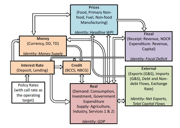
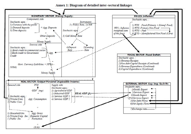
| RBI Working Paper Series No. 03 Abstract 1The paper develops a series of structural equations outlining relations within and across sectors of the macro-economy in India. The economy is conceived as a network of five sectors, the output (GDP and its components), prices (WPI and its components), monetary (money supply and interest rates), government finance (government expenditure and receipts) and the external sector (trade, capital flows and exchange rate). Estimations are made over 1980-81 to 2012-13 with annual data and at disaggregated levels so as to provide a clear idea about inter-linkages and channels of policy transmission in India. The emphasis is to understand the evolving economic structures in India over a long period of time. Variables are mostly in growth form (annual percentage change) and stationary that make it a useful framework of policy inferences. Equations are estimated using ordinary least squares with dummies taking into account regime changes and other known events. Using equations for forecasting may not be advisable as they reflect average relation over a long period of time with structural breaks. This can nevertheless be useful as preliminary work for a macro-model in India. JEL Classifications: E1; E2; E3; E4 Keywords: India; Macro-aggregates; Sectoral Dynamics; Inter-sectoral Linkages Section I: Introduction Empirical research to back macro-model in India is limited. The prominence of research for forward looking economic assessment including model building and policy simulation is now emphasised and institutionalised within the RBI. In this context, this paper estimates a set of structural equations so as to enable further work on macro-model in India for its use in monetary policy. The paper is arranged as follows. Section II outlines motivation of the study. A brief overview of structural linkages is presented in Section III. Estimation details are given in Section IV. Concluding observations are made in Section V. Section II: Motivation for this Study Econometric models covering sub-sectors of the Indian economy date back to the mid-1950s. Earlier models (until 1960s) confront with data problems [Narasimham (1956), Krishnamurty (1964)]. As more data are available, models become disaggregated (in the 1970s) with added focus on policy analysis [Pandit (1973), Pani(1977) and Chakrabarty (1977)]. Models of the 1980s step up policy focus further. P.K. Pani (1984) analyzes structural equations for output, demand, fiscal operations, money supply and prices. Chakrabarty (1987) establishes linkages among real, fiscal, monetary and external sectors over 1962-63 to 1983-84. Rangarajan, Basu and Jadhav (1989) examine interaction between government deficit and debt. Rangarajan and Singh (1984) analyze reserve money multiplier. Pradhan, Ratha and Sharma (1990) explore the interaction between the public and the private sector. The models in the 1990s address more complex issues in the wake of economic reforms [Chakrabarty and Joshi (1994), Rangarajan and Mohanty (1997) and Klein and Palanivel (1999)]. Rangarajan and Arif (1990) ascertain differential impacts of monetary expansion on output and prices in a state of less than full employment. Rangarajan and Mohanty (1997) focus on macroeconomic impacts of fiscal deficit. Besides individual attempts, there are institutional attempts to build and maintain comprehensive models for policy analysis and generating forecasts. Economic and financial integration with the global economy become an important channel of disturbance for the Indian economy over the last two decades. Accordingly, a need for econometric model arises linking all the important sectors of the Indian economy (Krishnamurty, 2002). Singh (2005) designs an econometric model covering 1985–1986 to 2001–2002. Patra and Kapur (2010) use a New-Keynesian framework to understand inflation. None of these models however deals with the rapid institutional and structural changes in the Indian economy. Econometric models are also undermined by the lack of comprehensive and consistent database in India. Monetary policy making within the RBI pursues various ad-hoc modelling efforts for forward looking assessment including the risks to growth and inflationary outlook. Such initiatives have been increasingly supplemented by more frequently available information like various leading and coincident indicators, company finance data, macro data on real, monetary, financial and fiscal parameters as also various survey results. The technical model based results are generally cross-checked against all other information for an overall consistency. With the RBI moving towards formal and flexible inflationary mandate, econometric modelling requirements are expected to take a more structural economy-wide base. This would call for a greater understanding of the interaction among variables and conducting a more comprehensive assessment of macro-risk scenarios in modelling/forecasting exercise. In this context, a revisit of the macroeconomic linkages within and across sectors is useful. Accordingly, this paper estimates several structural equations on a disaggregated dataset to explore how various sectors across the macro-economy relate within and among themselves, the importance of variables in explaining others and the ways their impact is likely to percolate through the overall economic structure in India. Although the larger aim is to fill the existing gap of econometric modelling in India, the approach here is to use a simple and flexible estimation framework, while capturing all important information. It is expected to aid in an understanding of all the major sub-sectors and create a base for further research and more sophisticated analysis on the macro-economic outlook in the future. Section III: A Brief Overview of the Structural Linkages A set of equations are estimated to explore linkages amongst important macroeconomic variables across: (i) Monetary, (ii) Prices, (iii) Real, (iv) Fiscal, and (v) External sectors. Each sector can technically be described through an array of behavioural equations and identities. Although identities are not appearing directly in the estimations, they are still necessary to understand the vital links among equations. Owing to a long estimation period, there are many structural breaks and known events in the data that are controlled for consistent estimates under this framework. The disaggregation in the model reveals a detailed transmission network and stylised trend over a period of time which can be summarised as follows. Monetary policy impulses appear through policy instrument/interest rates affecting the money market rate, which then transmits through a broader spectrum of deposit and lending rates. It also affects credit conditions in terms of deposit and credit growth and the real economy in terms of GDP growth and WPI inflation. Fiscal condition impacts lending rates by changing the level of private sector borrowings. The impact of credit cost on private investments is also prominent. The monetary policy variables like money growth and interest rate affect non-food manufacturing inflation at the wholesale level, which was often interpreted as core inflation by monetary authorities in India until the very recent period. India’s global integration and gradually market determined exchange rates are having notable impact on several components of WPI inflation. Exchange rate affects prices directly through imported goods and has an indirect impact too through net exports and real GDP. The broad linkages in the model have been shown as Figure 1. A more detailed description is provided in Annex 1. The growth of real GDP and prices impact many other variables in the fiscal and external sector equations. For instance, the revenue growth of government as also government’s capital expenditure shows higher pro-cyclicality both in terms of growth and inflation rates. Revenue expenditure on the other hand is relatively sticky and shows mild pro-cyclicality. It is also observed that government’s ability to spend depends on its cost of borrowings to a significant extent. As regards external sector, separation of India’s exports and imports to goods and services components offers some important insights. India’s services output growth shows a far greater influence on India’s services exports growth as compared with a similar impact of the manufacturing output growth over the merchandise exports. In respect to global income elasticity of India’s exports, it is observed that services exports exhibit relative resilience to the global growth cycle as opposed to merchandise exports showing larger movements in response to the same. India’s imports of goods and services also show very high elasticity in response to domestic activities. In comparison, the impact of real exchange rates on both exports and imports is rather small. Instead, relative changes in the nominal Rupee movements vis-a-vis other currencies convey information regarding the path of external trade and capital flows. Debt and equity inflows are estimated separately by reclassifying items in the balance of payments accounts, which depend on a separate set of factors. A more elaborated description of the model is presented as Annex 2. Estimations are made over 1980-81 to 2012-13 with annual data. Variables are chosen mostly in the growth form (annual % change), which is usually closely monitored by the RBI. All variables are tested to be stationary, except for some ratios and rates that make it a useful framework for making key inferences. Owing to a long estimation period, there are however many structural changes and regime shifts in the data. Accordingly, equations are estimated using ordinary least squares with appropriate dummies. An overall view of the macro-aggregates can be arrived at by using them in a forecasting framework. However, it may be difficult as estimations are made over a very long period of time with many structural breaks. Therefore, the exercise can be viewed more as a tool for understanding policy transmission in India and could be useful for certain inferences. Section IV: Estimates of the Equations Specifying equations in an OLS framework is a cumbersome task given the expected endogeneity among variables. Endogeneity can come from various sources like having a common trend, simultaneity in relations, impact of a common structural break, common measurement error in variables, etc. In view of the possible co-integration among variables, we chose to explore relations only on the de-trended data. Accordingly, all variables have been converted into growth rate and ratios to ensure that the resultant variables are stationary, which is mostly satisfied. We stick to the OLS as it is easy to understand, flexible to use and offers important insights about the functioning of the economy through appropriate mapping of the relationship. Equations are specified in a way to avoid simultaneity bias to the extent possible. Where endogeneity is suspected, we tried estimating the equation using 2SLS, which in all the cases gave similar outcomes. Explanatory variables in certain equations were tested for endogeneity and incorporated only after they satisfy the test. Finally, most of the structural breaks in the data due to known events are handled through dummy variables. Overall, OLS appears to be a reasonable approximation. Variables in the equations are incorporated in a theoretically consistent manner and at a disaggregated level. For instance, in the monetary sector, the sum of currency with the public, demand and time deposits together constitute the money supply from the components side, each of them having a separate equation. From the sources side, we estimate equations for credit to the commercial sector and Government separately. In explaining prices, we disaggregate meaningful sub-components of WPI and explain each of them separately for their overall impact. Accordingly, WPI Inflation has been seen as the sum of Food (both primary and manufactured food), Fuel, Non-food Primary Articles and Non-food Manufactured Products. Similarly, GDP growth is estimated from both the demand as well as the supply sides to understand the drivers of sub-components. The demand side estimations involve consumption and investment, while components of net exports and government spending are dealt in the external and fiscal sector, respectively. Both consumption and investment equations are developed at more disaggregated levels. The components of GDP from the supply side are viewed as the sum total of sectoral outputs emanating from agricultural, industrial and services that are explained by a different sets of variables. The services GDP is further sub-divided into services excluding community and personal services (services 1) and services 2 accounting for only the community and personal services, the latter exhibiting different characteristics than the rest of the services sector. Similarly, various items of revenue and capital accounts have been estimated separately in the fiscal sector. In the external sector, we separated merchandise and services both for imports and exports and also segregated debt and equity within the overall external capital flows. Sector-wise behavioural equations and identities in the model are presented as Annex 2. Estimations are made over the sample period 1980-81 to 2012-13 with annual data. Expansion of the dataset beyond 2012-13 proves to be difficult in view of the new GDP series that has quite a different sectoral composition. Variables are mostly in growth form (annual % change), apart from a few ratios (e.g., dependency ratio, fiscal deficit to GDP ratio, CAD to GDP ratio, etc.) and rates (e.g., various interest and exchange rates). Differencing these variables could lead to a loss of information besides complicating their interpretations. This could however influence the stability of the parameters. Thus, all the equations have been tested for standard diagnostic checks to ensure absence of autocorrelation in residuals (Correlogram Q-statistics/Serial correlation LM tests) and for the stability of the parameters (i.e., CUSUM/CUSUM of Square tests) (Annex 3). Sector 1: Monetary Sector Development of the monetary sector avoids complications relating to shifts in the monetary policy over the period in terms of different policy instruments as also changes in the emphasis of monetary operation. Instead of using multiple monetary policy instruments, we prefer using an effective policy rate series by combining various instruments along with reserve requirements. Issues like the role of asset prices in monetary policy transmission or the shift in targeting of an inflation rate by the RBI is not incorporated. Monetary aggregates are seen mostly from an accounting framework with each equation explaining trends of disaggregated variables within the broader components and having a distinct behavioural relation from others. Apart from quantity variables, there are different interest rate variables within the monetary sector. Among them, the overnight call rate is expected to reflect both the quantity and price based monetary policy signals. The deposit and lending rates, on the other hand, are expected to reflect policy rate transmission through a change in the cost of funds. 1.1 Currency with the Public (M3 data) Currency= f [Disposable income, Deposit rate, Dummies] Currency with the public reflects transaction demand responding to personal disposable income as well as substitution effects responding to the deposit rates. A few dummies have been used to get rid of outliers. Currency demand is positively associated with income and negatively associated with the interest rate on deposit reflecting the opportunity cost of holding money. 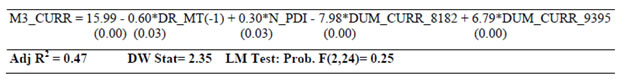 Variables: M3_CURR: growth in currency with the public, DR_MT(-1): one period lag in interest rate on deposits of 1-3 year maturity, N_PDI: growth in nominal personal disposable income, DUM_CURR_8182 is a dummy for 1981-82 to take into account sharp deceleration in currency growth and DUM_CURR_9395 is a dummy variable for the period 1993-95 to take into account the sharp increase in currency growth. 1.2 Demand Deposits (M3 data) Demand Deposits = f [GDP, Own lags, Dummies] Demand deposit mostly reflects the transaction demand for money from a broader economic perspective. Real GDP growth influences the growth in demand deposits in India positively and significantly. 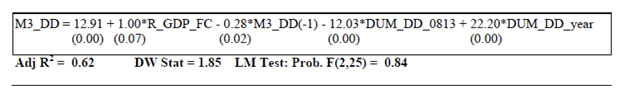 Variables: M3_DD: growth in demand deposits, R_GDP_FC: real GDP (at factor cost) growth, M3_DD(-1): one period lagged growth in demand deposits, DUM_DD_0813 is a dummy variable for the period 2008-09 to 2012-13 to take into account the crisis impact when its growth has fallen and DUM_DD_year is a dummy for years 1991-92, 1994-95 and 2005-06 to take into account the strong growth in demand deposits. 1.3 Time Deposits (M3 data) Time Deposits = f [Disposable income, Deposit Rate, Inflation, Alternative Returns, Dummies] Time deposits reflect the income effect, its lagged return (to the extent that deposit tenors are relatively long in India), return on alternate assets like equity and administered interest rates on various small savings schemes in India. 1-3 year deposit rate has been used as the representative rate. Lagged WPI inflation reflects expected inflation and therefore indicates flight of funds to high yielding instruments outside the banking sector. PPF rate impacts time deposit growth statistically significantly by offering a competing product for time deposits. On the other hand, term deposits are not influenced by returns on equity latter being an imperfect substitute for bank deposits. 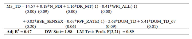 Variables: M3_TD: growth in time deposits, N_PDI: growth in nominal personal disposable income, DR_MT(-1): one period lag in interest rates on 1-3 years deposits, WPI_ALL(-1): one period lagged WPI inflation rate, BSE_SENSEX: growth in benchmark stock index of BSE e.g. SENSEX, PPF_RATE(-1): one period lag in interest rate on provident funds, DUM_TD_67 takes value 1 for the year 2006-07 on account of sudden drop in deposit growth and DUM_TD is a dummy variable with values 1 for 1990-91 and 1995-96 to take into account the effect of stabilisation and structural adjustments in India on term deposit of banks. 1.4 Bank Credit to Commercial Sector (M3 data) Bank Credit to Commercial Sector = f [GDP, Aggregate deposits, Inflation, Lending rate, Net Bank Credit to Govt., Dummies] Bank credit to commercial sector reflects underlying real activity as captured here through GDP growth, state of resource availability through aggregate deposits growth, the real cost of borrowing (real SBI advance rate) and diversion of resources through growth in net bank credit to the central government. As is evident here, lower real lending rate or even higher inflation reduces borrowing costs in real terms enabling larger demand for credit. The negative sign of growth in net bank credit to central government indicates greater impounding of resources by the government reduces the availability for the private sector. 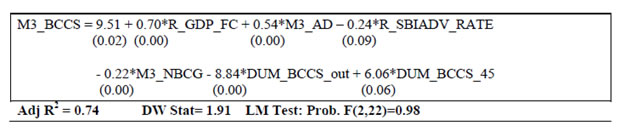 Variables: M3_BCCS: growth in bank credit to commercial sector as in M3 data, R_GDP_FC: growth in real GDP, M3_AD: growth in aggregate deposits, R_SBIADV_RATE: Real SBI advance rate, DUM_BCCS_45 is a dummy variable with value 1 for the year 2004-05 to reflect sudden spike in credit and DUM_BCCS_out is a dummy variable with values 1 for the years 1990-91 (gulf crisis), 1993-94 (immediately after the BOP crisis), 1996-97 (slowdown in industrial growth) and 2003-04 to take into account the outliers in data. 1.5 Net Bank Credit to Central Government (M3 data) Bank Credit to Central Govt. = f [Centre’s Gross fiscal deficit, Own lag] Growth in net bank credit to central government captures the impact of large size and persistence of fiscal deficits in India. The positive lagged coefficient implies persistence in the growth in net bank credit to government. Although RBI stopped accommodating direct government borrowings in recent years, a large fiscal deficit inevitably supplies government papers in the financial market, a part of which is held by banks. Banks can also use those papers as collateral to borrow from the RBI. 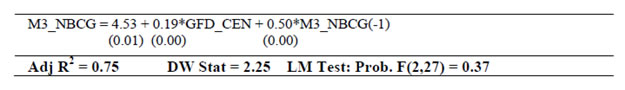 Variables: M3_NBCG: growth in net bank credit to government as in M3 data, GFD_CEN: growth in the level of gross fiscal deficit of centre, M3_NBCG(-1): growth in net bank credit to central government lagged by one period. 1.6 Interest Rate: Call Money Rate Call Rate = f [Effective policy rate, CRR, Dummies] Movements in call rate should reflect the dynamics of the demand and the supply of overnight liquidity intermittently affected by policy signals of the monetary authorities. The operating framework of such policy signals, although varies from time to time, can nevertheless be considered emanating from an effective policy rate series computed by us combining the Bank Rate and weighted LAF repo/reverse repo rates (weights being the volumes of repo and reverse repo bids accepted). Reserve demand, on the other hand, largely derives from the level of Cash Reserve Ratio (CRR) specified by the RBI from time to time. Supply of reserve mostly emerges from liquidity operations by the central bank. In fact, if proxies for RBI’s operations in the forex and domestic markets are introduced into the equation, the coefficient of policy rate becomes higher. The impact of such liquidity management operations themselves however turns out insignificant. On overall balance, the specified equation shows greater impact of the weighted policy rate changes on call rate than the CRR changes. However, the estimates are sensitive to the measures of average policy rate used. When simple average policy rate (average of LAF repo and reverse repo) was used, the impact of CRR changes goes up. 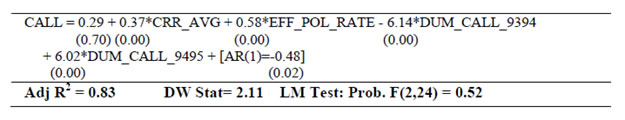 Variables: CALL: Weighted average call money rate, CRR_AVG: average of the applicable CRR (CRR changes) during the year, EFF_POL_RATE: effective policy interest rate which is a combination of Bank Rate from 1980-81 to 2000-01 and weighted average of LAF reverse repo and repo rate during 2001-02 to 2012-13 (weights being the reverse repo/repo amounts), DUM_CALL_9394 and DUM_CALL_9495 are two dummy variables to take into account unusual fall in call rate in 1993-94 and unusual increase during 1994-95, respectively. 1.7 Interest Rate: Deposits Rate (1-3 year maturity) Deposit Rate= f [Call rate, Own lag, Dummies] Deposit rate reflects the pass-through of policy rate changes through call rate. Such pass-through is sluggish and therefore, a degree of its persistence is added to account for slow adjustments. The equation, in fact, shows stronger persistence of deposit rate and relatively lower pass-through from call rate to deposit rate. In fact, if lagged call rate is introduced, the contemporaneous effect of call becomes insignificant. On balance, we consider that the current formulation is realistic to reflect the fact that policy transmissions are in fact sluggish and weaker. 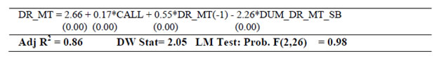 Variables: DR_MT: interest rate on deposits of 1-3 years maturity, CALL: weighted average call money rate, DR_MT(-1): interest rate on deposits of 1-3 years maturity lagged by one period, DUM_DR_MT_SB: dummy variable to take into account the sharp fall in interest rates in 2002-03 and 2003-04 owing to strong capital flows. 1.8 Interest Rate: Lending Rate (proxied by SBI advance rate) Lending rate = f [Call rate, Inflation, Fiscal deficit, Own lag, Dummies] Lending rate too reflects the pass-through of policy rate changes through call rate, inflation rate, persistence and the large size of fiscal deficits in India. Like deposit rates, lending rate shows a higher degree of persistence as compared to observed transmission from money market rates. Unlike deposit rates, higher inflation rate and fiscal deficit of the centre puts some upward pressure on lending rates in India. 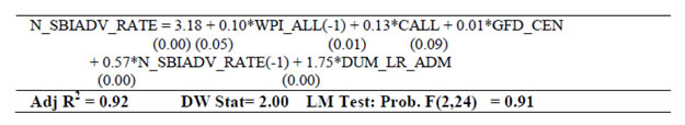 Variables: N_SBIADV_RATE: SBI advance rate as the proxy for lending rate, WPI_ALL(-1): Lagged WPI annual inflation rate, CALL: weighted average call money rate, GFD_CEN: growth in amount of gross fiscal deficit to centre, SBIADV_RATE(-1): SBI advance rate lagged by one period, DUM_SBIADV_ADMN: dummy for the administered interest rate regime when SBI advance rate was fixed during 1980-81 to 1993-94 (=1) Sector 2: Prices Sector The recent shift in the nominal anchor of monetary policy with explicit focus on the consumer price inflation rate enhances the need for understanding the inflationary processes in India. The following set of equations, however, does not reflect this transition. As equations are developed for a long period, it would not be possible to capture such contemporary developments. Instead, we rely on WPI inflation, which monetary authority in India has considered as the relevant price indicator until the very recent period. WPIs are computed for its four sub-components- Food (weight – 24.3 per cent; combining primary food and manufactured food products), Primary Non-food (weight – 5.8 per cent; combining primary non-food articles and minerals), Fuel Group (weight – 14.9 per cent), and Non-food Manufactured Products (weight– 55.0 per cent; manufactured products excluding food items). 2.1 WPI – Food WPI-Food = f [GDP (Agri), Rainfall, MSP, Global Food Prices, GDP (Non-Agri)/PFCE (Food), Dummies] WPI food inflation seeks to capture the impact of both the demand and the supply factors as also the level of global food prices. On the demand side, growth in private final consumption expenditure on food is used as a measure of demand for food in India. Expenditure on food as a proportion of non-agricultural income has fallen steadily in India from close to 75 per cent to under 20 per cent over 1970 – 2012 consistent with economic growth and consequent compositional shifts in the food basket emphasized in the theoretical and empirical literature. Composition of demand within food also shifted from lower value cereals to higher value protein products, with consequent inflationary impact. On the supply side, we use lagged agricultural GDP, rainfall, drought conditions and minimum support price for food items as the relevant explanatory variables. We incorporate rainfall in addition to drought conditions to account of the fact that the overall magnitude of rainfall often fails to capture its spatial and temporal distribution and therefore, its fuller impact on the agricultural output and prices. The Minimum Support Price (MSP) of food derived from the cost of production is known for setting a floor to food prices. Both the demand and the supply side variables along with MSP are statistically significant. International food prices are also significant, even though the magnitude is somewhat smaller. Global and domestic food prices in India moved together till 2000. Subsequently, global food prices turned volatile, while food prices in India saw secular rise, perhaps reflecting changing demand for protein related food items. The same phenomenon is controlled for in the equation by using dummies. 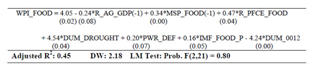 Variables: WPI_FOOD: Annual Inflation in WPI – Food; R_AG_GDP(-1): Lagged annual % change in Real Agricultural GDP; MSP_FOOD(-1): Lagged annual % change in MSP of Food (Paddy, Wheat, Coarse Cereals and Pulses); R_PFCE_FOOD: Annual % change in Private Final Consumption Expenditure on Food at 2004-05 Prices; DUM_DROUGHT: 1991, 1997, 2002 - the years when decline in real agricultural GDP was of the order of 2 per cent or more; PWR_DEF: Production-weighted rainfall deficit; IMF_FOOD_P: Annual % change in IMF’s food price index; DUM_0012: for 2000-01 to 2011-12, when domestic food prices notably diverged from the global prices. 2.2 WPI – Fuel and Power WPI-Fuel = f [Global crude price, Rs/US$ Exchange rate, Real GDP growth] WPI inflation in the Fuel group is largely driven by international crude prices because India imports over 80 per cent of its total requirement of crude oil. We used IMF’s crude oil price index as one of the explanatory variable for global price, which is highly significant in the equation. In addition to the international prices, the landed cost of crude oil also depends on Rupee-Dollar exchange rates, which is also significant. There is an evidence of less than full pass-through as 1 percentage point depreciation of Rupee-US Dollar rate leads to only 0.21 percentage point increase in fuel prices as WPI Fuel group also consists of commodities characterized by administered pricing. 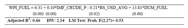 Variables: WPI_FUEL: Annual Inflation in WPI – Fuel and Power; IMF_CRUDE_P: Annual % change in IMF-Crude Oil Prices (USD/barrel); RS_USD_AVG: Average Rupee-Dollar Rate; DUM_ FUEL: 1980, 1981, 1993, 2000 – years for which WPI – Fuel and Power increase was in excess of 15 per cent 2.3 WPI – Primary Non-food WPI-Non-food articles = f[Global Non-food Primary Prices, Exchange Rate, Demand, Dummies] Primary non-food is the most volatile component within the WPI as it consists of industrial inputs with significant trade links. We use global vegetable oil index (for WPI oilseeds) and global agricultural raw material index as explanatory variables with limited success. Nominal effective exchange rate also played an important role. 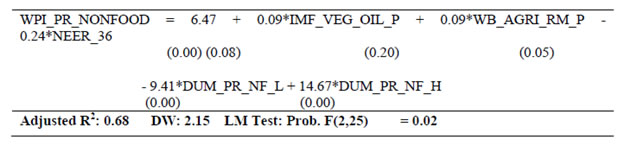 Variables: WPI_PR_NONFOOD: Annual Inflation in WPI – Non-food; IMF_VEG_OIL_P: Annual % change in IMF’s Commodity Vegetable Oil Index; WB_AGRI_RM_P: Annual % change in World Bank’s Agricultural Raw Material Price Index; NEER_36: Appreciation(+)/ Depreciation(-) in Nominal Effective Exchange Rate; DUM_PR_NF_H: 1980, 1994, 2010; DUM_PR_NF_L: 1985, 1988, 1999 2.4 WPI – Non-food Manufactured Products WPI-NFMP = f[Output gap, Policy Rate, Money supply, Exchange rate, Global crude prices, Dummies] The Non-food Manufactured Products is regarded as the core component within the WPI inflation and therefore is expected to be affected by some measure of aggregate demand. Output gap, most widely used measure of economic cycles, however fails to yield a statistically significant coefficient. Money supply gap, on the other hand, turns out to be the significant determinant of aggregate demand pressure. This possibly suggests that output expansion, only if accommodated by monetary growth, is inflationary in India. IMF’s crude oil price and nominal effective exchange rate are observed to be other important determinant through cost of import channel. The dummy for the period 1996-2012 takes into account a structural downward shift in core inflation in India in line with the great moderation in the global price trends. 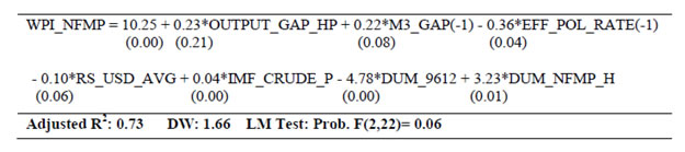 Variables: WPI_NFMP: Annual Inflation in WPI – Non-food Manufactured Products; OUTPUT_GAP_HP: Output Gap calculated using the Hodrick-Prescott filter, M3_GAP(-1): one period lag in money gap (deviation from projected M3 growth announced in policy); EFF_POL_RATE(-1): effective policy interest rate which is a combination of Bank Rate from 1980-81 to 2000-01 and weighted average of LAF reverse repo and repo rate during 2001-02 to 2012-13 (weights being the reverse repo/repo amounts); RS_USD_AVG: Average Rupee-Dollar Rate; IMF_CRUDE_P: Annual % change in IMF-Crude Oil Prices (USD/barrel); DUM_9612: Dummy for the period 1996-2012, DUM_NFMP_H: 1991, 1992, 1994 – years when Non-food Manufactured Inflation exceed 10%. Sector 3: Real Sector In the real sector, GDP growth is estimated from both the production (real GDP at factor cost) and demand side (real GDP at market prices), even though independent demand side estimates of GDP in India are not of very good quality. Nevertheless, demand side variables of GDP offer several insights about the possible transmission channels of economic activities. Sector 3.1: GDP from the Demand Side Consumption is estimated separately for private and government entities, while investments are estimated across classes of economic agents such as the households, private corporate sector and the government. 3.1.1 Private Final Consumption Expenditure Pvt. consumption = f [Personal disposable income, WPI inflation, Dependency ratio, Deposit rate, Wealth effect, Persistence effect and Dummies] Private Consumption is obtained as a function of real Personal Disposable Income, Dependency Ratio of population and returns from a few financial asset consistent with established economic theories. Some of the important determinants of consumption observed in empirical work internationally like time preference, wealth, age structure, etc., failed to obtain expected results in India. 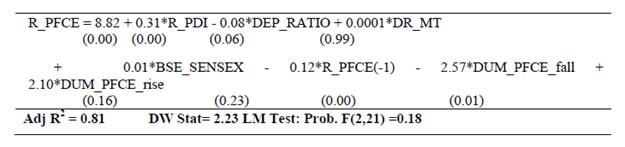 Variables: R_PFCE: Growth in real private final consumption expenditure (at market prices); R_PDI: Growth in personal disposable income ( at constant prices); DEP_RATIO: Age dependency ratio (Dependent population as % of working-age population); WPI_ALL: Inflation rate (All Commodities); DR_MT: Deposit rate 1 to 3 years; BSE_SENSEX: growth in benchmark stock index of BSE e.g. SENSEX; R_PFCE(-1) : one period lag in R_PFCE; DUM_PFCE_rise: Dummy variable for years in which PFCE registered unusual rise e.g. 1980, 1983, 1996 and 2005-2011; DUM_PFCE_fall: Dummy variable for years in which PFCE had fallen sharply e.g. 1982 and 1992. 3.1.2 Government Final Consumption Expenditure Govt. consumption = f [Combined primary revenue expenditure, Inflation, Dummies] Government Consumption Expenditure is estimated through Primary Revenue Expenditure for central and state government together besides using WPI Inflation Rate. As the combined revenue expenditure of the government is more predictable and budgeted ahead, it can possibly be used as an indicator to assess the likely levels of real government consumption expenditure a year ahead. Higher inflation rate reduces government discretionary consumption possibly through a rise in committed non-plan expenditure like subsidy, interest burden, etc., leaving lesser room for adjustments without pushing up fiscal deficit commensurately. More insights on these would be available in the fiscal sector of the estimated equations. 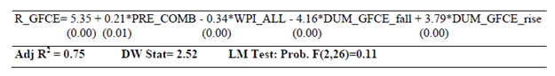 Variables: R_GFCE: Growth in Real Government Final Consumption Expenditure (mp); PRE_COMB: Growth in Combined Primary Revenue Expenditure of Centre and States; WPI_ALL: Inflation rate; DUM_GFCE_rise: Dummy variable for years in which GFCE rose abruptly as possible fiscal stimulus, e.g. 1985, 1997, 1998, 1999, 2005, 2008, 2009; DUM_GFCE_fall: Dummy variable for years in which GFCE had fallen sizeably e.g. 1991 and 2000, 2001 and 2002. Investments - the Overall Estimation Framework Investment equations are estimated separately for Household, Private Corporate and Public Sector. Of late, the household sector accounts for 39 per cent of the gross domestic capital formation net of valuables, followed by private corporate sector (33 per cent) and public sector (22 per cent). The average growth of investment during 1980-2011 for private corporate sector has been 14.5 per cent, followed by household investment growth at 10.1 per cent and public sector investment growth at 5.6 per cent. Higher volatility in investment rendered these estimations quite difficult. Among various sectors, private corporate sector investment shows highest volatility (standard deviation of investment growth), while public sector investment the least. Going by the standard economic theories, investment demand, prima facie, should respond to economic cycles, stock market valuation and expected profitability. However, only financial repression emerges as the most prominent determinants of investments in India. Economic cycles reflected in investment demand only when such rise in demand is either accompanied by adequate accommodation of credit (in case of private corporate business) or facilitated by public investments. Investment climate proxied by equity returns turns out to be statistically significant only for corporate sector. 3.1.3 Household Sector Investment Household investment = f [Personal Disposable Income, Lending Rate, Dummies] Household sector investment is determined by real personal disposable income growth, real cost of borrowings and WPI inflation. Access to credit remains insignificant perhaps because a large part of investments by households in India is self-funded and thus investment is explained by the real personal disposable income growth. Real PDI growth also facilitates household investments consistent with the hypothesis of improved cash flow removing financial constraints to household investments. Higher inflation perhaps reduces profitability and enhances investment uncertainty of household/SMEs, and thereby observed to be holding back investments. 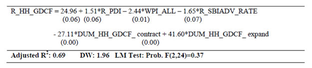 Variables: R_HH_GDCF: Growth in Real Gross Domestic Capital Formation of the Household Sector; R_PDI: Personal Disposable Income at Constant Price; WPI_ALL: WPI Inflation; R_SBI_ADV_RATE: Real SBI Advance Rate; DUM_HH_GDCF_ expand: Dummy for 1983, 1987, 1995 and 1997 – high growth years of household investment; DUM_HH_GDCF_ contract: Dummy for 1991 and 1996 – marked contraction years of household investment. 3.1.4 Private Corporate Sector Investment Pvt. Corporate Investment = f [Bank Credit, Real Lending Rate, Investment Climate, Own Lag] Access to non-food bank credit improves investment in private corporate sector remarkably. The impact of real leading rate is also clearly evident and more so in the relatively recent period (since 1992) as interest rates have been deregulated. 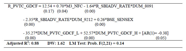 Variables: R_PVTC_GDCF: Growth in Real Gross Domestic Capital Formation of the Private Corporate Sector; M3_NFC: Non-food Credit; R_SBIADV_RATE: Real SBI Advance Rate (Nominal minus WPI Inflation); R_SBIADV_RATE*DUM_8091: Dummy for the period 1980-1991 when interest rates were mostly administered; R_SBIADV_RATE*DUM_9212: Dummy for the period 1992-2011 during which interest rates were gradually deregulated; BSE_SENSEX: Growth in BSE Sensex; DUM_PVTC_GDCF_H: Dummy for 1981, 1995 and 2004 – abnormally high growth years of private corporate investment; DUM_PVTC_GDCF_L: Dummy for 1983, 1987, 2000, 2008 and 2011 –high contraction years. 3.1.5 Public Sector Investment Public Sector Investment = f [Combined capital expenditure, GDP Cycle, Dummies] Public sector investment is facilitated by real combined capital expenditure of Centre and States together. The cyclically adjusted real GDP growth has large explanatory power owing to the predominant presence of public investment in the infrastructure sector that is possibly accommodated during economic expansion in terms of large expenditures on public investments. 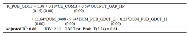 Variables: R_ PUB_GDCF: Growth in Real Gross Domestic Capital Formation of the Public Sector; CE_COMB: Growth in Real Capital Expenditure of the Centre and State Combined; OUTPUT_GAP_HP: Cyclical component of growth in Real GDP; DUM0408: Dummy for high growth period of 2004-08; DUM_PUB_GDCF_H: Dummy for 1981, 1994 and 1999 –high growth years of public sector investment; DUM_PUB_GDCF_L: Dummy for 1987 and 1995–high contraction years of public sector investment. Sector 3.2: GDP from the Supply Side GDP growth is viewed as the sum total of output originating from agriculture, industry and services separately. Services is further broken down to pure government services such as community, social and personal services (named as Services 2) and services excluding community, social and personal services (named as Services 1) in view of their separate characteristics. 3.2.1 Real Gross Domestic Product in Agriculture and Allied Sector Agricultural output = f [Area under cultivation, Capital formation, Fertilizer consumption in agriculture, Rainfall, Agricultural credit, Demand, Dummies] Growth in real agricultural output reflects both the supply and the demand side factors. From the supply-side, variables like growth in total area under cultivation (TAUC), deviation in production-weighted rainfall from its 10-year average rainfall (PWR_DEV) and agricultural credit is important. On the demand side, growth in real private final consumption expenditure scales up agricultural output perhaps because it enables shifts in agricultural output towards high value products. A dummy is introduced to capture outliers emerging from strong growth in agricultural output following the instances of agricultural failure, especially in the drought years. 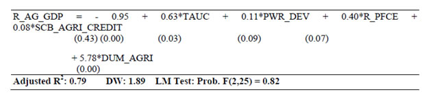 Variables: R_AG_GDP: Real GDP in Agriculture and Allied Sector; TAUC: Total Area under Cultivation Index; PWR_DEV: Positive deviation of Production Weighted Rainfall from rolling 10-year average rainfall; R_PFCE: Real Private Final Consumption Expenditure; SCB_AGRI_CREDIT: Sectoral Deployment of Credit to Agriculture; DUM_AGRI: Dummy for 1988, 1992, 1996. 3.2.2 Real Gross Domestic Product in Industry Industrial Output = f [Gross investment, Lending rate, REER, Global IIP, Own lag, Dummies] Industrial GDP is estimated using overall capital formation, real interest rate, real exchange rate and cost of borrowing (real SBI advance rate). Although manufacturing segment within the industrial sector often behaves differently as compared to other segments, estimation of headline industrial output growth is attempted without further disaggregation to limit the number of equations in real sector. 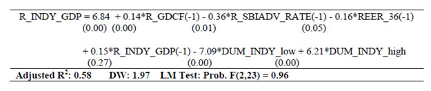 Variables: R_INDY_GDP: Real GDP in Industry; R_GDCF(-1): One period lag of Real Gross Domestic Capital Formation; R_SBIADV_RATE(-1): One period lag of Real SBI Advance Rate (Nominal minus WPI Inflation); REER_36(-1): One period lag of Real Effective Exchange Rate; R_GDP_INDY(-1): One period lag of Real GDP in Industry; DUM_INDY_low: Dummy for 1991, 2011 and 2012; DUM_INDY_high: Dummy for 1994 and 2006. 3.2.3 Real Gross Domestic Product in services sector 1 (excluding community & personal) Output in services sector 1 (ex-community & personal) = f [Own lag, private income, primary expenditure, industrial output, Services export, lending (SBI advance/call) rate)] The Real GDP for Services excluding Community and Personal Services (R_GDP_SERV1) reflects the impact of real interest rate, real personal disposable income, services exports, exchange rate besides its own lag and some dummies. The lagged real PDI suggests sensitivity of services output to demand. Observed large lagged co-efficient as opposed to industrial output reflects higher persistence of services GDP growth as compared with industry GDP growth. 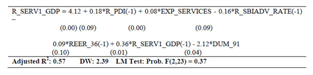 Variables: R_GDP_SERV1: Real GDP in Services Sector 1 (ex community and personal); R_PDI(-1): One period lag of Real Personal Disposable Income; SERV_EXP: Services Export; R_SBIADV_RATE(-1): One period lag of Real SBI Advance Rate (Nominal minus WPI Inflation); R_GDP_SERV1(-1): One period lag of Real GDP in Services Sector 1 (ex community and personal); REER_36(-1): One period lag of Real Effective Exchange Rate; DUM_1991: Dummy for 1991. 3.2.4 Real Gross Domestic Product in services sector 2 (i.e., community, social & personal) The Real GDP for Community, Social and Personal Services reflects provision for services by the government and thus is estimated using lagged primary revenue (i.e., excluding interest payments) expenditure of the combined centre and state governments. As budget estimates of the primary revenue net of interest payments are available a year in advance, it can be used to assess the level of services output of the Community, Social and Personal Services. 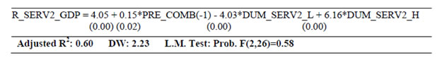 Variables: R_GDP_SERV2: Real GDP in Services Sector 2 (i.e., community, social and personal); PRE_COMB(-1): One period lag of Combined Primary Revenue Expenditure of Centre and States; DUM_SERV2_L: Dummy for 1981, 1991 and 1994; DUM_SERV2_H: Dummy for 1999 and 2008. Sector 4: Fiscal Sector Fiscal equations are estimated separately for revenue receipts, revenue expenditures, non-debt capital receipts and capital expenditures for the consolidated central and state governments’ budgets. Observed stickiness in government expenditures growth is captured through persistence parameter. Notwithstanding that, fiscal consolidation between 1997 and 2008 enables some improvement in the quality of government spending that is controlled for in the estimation. While revenue expenditure remains sticky, the burden of adjustments is borne by the capital expenditure, which fell from late 1980s to late 1990s before stabilizing at a lower level. Fiscal consolidation coincides with a general fall in inflation and reduction in the cost of borrowings by governments, also aiding to the containment of revenue expenditure. We have tried to estimate these phenomenon in this set of equations. 4.1 Revenue Receipts (Combined) Revenue Receipts (Comb.) = f (Real GDP, Inflation, Own lag, Dummies) Revenue receipt reflects current and previous years’ GDP growth and contemporaneous WPI inflation rates. 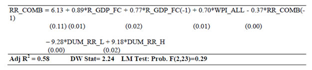 Variables: RR_COMB: growth in revenue receipts of the centre and states combined, R_GDP_FC: Real GDP growth, R_GDP_FC (-1): Real GDP growth lagged by one period, WPI_ALL: WPI inflation, RR_COMB(-1): growth in combined revenue receipts lagged by one period, DUM_RR_L is a dummy variable with values 1 for 1990, 1998, 2001 and 2008-09 to capture the impact of external crisis driven slowdown in revenue growth and DUM_RR_H is a dummy with value 1 for 1985 to capture the impact of very high growth. 4.2 Non-debt Capital Receipts (Combined) Non-debt Capital Receipts (Combined) = f [Past loans, Own lag, Dummies] Non-debt capital receipts mostly comprises recovery of past loans as well as disinvestment proceeds. Current year’s growth of non-debt capital receipt is linked to the loans and advances disbursed by the government 5 years back, equivalent to the median maturity of loans besides its own lag. 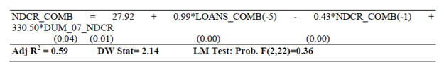 Variables: NDCR_COMB: growth in non-debt capital receipts of the centre and states combined, LOANS_COMB(-5): growth in combined loans and advances lagged by five period, NDCR_COMB(-1): one period lagged growth in non-debt capital receipts, DUM_07_NDCR is a dummy variable for 2007 to take into account the sharp increase in receipts on account of disinvestment proceeds. 4.3 Revenue Expenditure (Combined) Revenue Expenditure (Combined) = f [Real GDP, Inflation, Interest rate, Own lag, Dummies] Revenue expenditure equation intends to capture sensitivity to GDP growth and cost of borrowings (effective interest rate on Government’s borrowings) separately. In view of persistent nature of revenue expenditure, a lagged dependent term is also introduced. High persistence parameter in this equation shows a rather sticky revenue expenditure in real terms. It can be observed that higher growth enables government to finance higher revenue expenditure, while lower interest rates pushed expenditure up and vice versa. A comparison with 4.1 however reveals that output elasticity of revenue expenditure is lower as compared with revenue receipt. This suggests that the overall fiscal balance in India could be pro-cyclical. As against 4.1, there is however no evidence that inflation has direct contribution to the growth in revenue expenditure in a statistically significant manner. 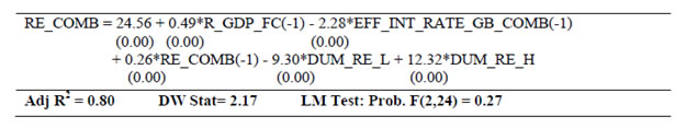 Variables: RE_COMB: growth in combined revenue expenditure, R_GDP_FC(-1): one year lagged GDP growth, EFF_INT_RATE_GB_COMB(-1): effective interest rate, which is derived as (interest payments/Combined liabilities lagged by one year)*100, RE_COMB(-1): one year lagged revenue expenditure growth, DUM_RE_L is a dummy variable with value 1 for 1981-82 to take into account an outlier in data and DUM_RE_H is a dummy variable with values 1 for the years 1998 and 2008 to capture the impact of pay commission awards. 4.4 Capital Expenditure (Combined) Capital Expenditure (Comb.)= f (Real GDP, Inflation, Own lag, Dummies) Capital expenditure of the combined government reflects higher sensitivity with respect to growth, while WPI inflation turns out to be insignificant. There has been a rise in capital expenditure during the periods of fiscal consolidation as reflected in the coefficient of DUM_CE_FRBM dummy. 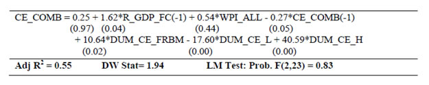 Variables: CE_COMB: Growth in combined capital expenditure, R_GDP_FC(-1): one year lagged real GDP growth, WPI_ALL: WPI Inflation, CE_COMB(-1): one year lagged capital expenditure growth, DUM_CE_FRBM is a dummy variable for the years 2001 to 2007 to capture the trend in capital expenditure during periods of fiscal consolidation, DUM_CE_L is a dummy variable with values 1 for 1989, 1995 and 2002 to capture the impact of sharp fall in growth of capital expenditure for reasons not controlled in this equation, while DUM_CE_H is a dummy variable with value 1 for 1986 to take into account its sharp growth. Sector 5: External Sector External sector has been estimated separately for the current and capital accounts as given below: Current Account Current account estimations are on merchandise (for goods exports and imports) and invisibles (services export and import) accounts separately. Real Effective Exchange Rate (REER) is taken as the proxy for measuring competitiveness of Indian exports. However, there are instances where current account balance fell sharply notwithstanding sharp exchange rate depreciation especially in 1991 Balance of Payments Crisis, 1997 Asian Crisis and 2008 sub-prime crisis. Also, India’s current account balance remains narrow or even in surplus despite sharp exchange rate appreciation during 2003-08. It is not possible to explain them by standard expenditure switching effects of exchange rate. Instead, the outlook of Indian Rupee against a broader set of currencies can be helpful to understand the underlying sentiments ruling the Rupee that is reflected in several current and capital account variables. In other words, while REER measures Rupee’s relative position from an international trade perspective, relative (un-weighted) nominal currency movements could have information about the outlook of the currency that goes beyond international trade. We construct a variable (RS_USD_AVG-USD_BROAD) to capture excess movements (appreciation/depreciation in % terms) of Indian currency over and above a broad set of other currencies (as included in US Broad Index) against the US Dollar. This is likely to reflect currency outlook of Indian Rupee relative to her global peer that could have an impact over the current and the capital accounts. RS_USD_AVG-USD_BROAD is included in addition to real exchange rate level (REER) in most of the equations to measure the relative currency movement of Rupee. 5.1 Goods Export Goods Export = f (World GDP, Manufacturing GDP, Real Exchange Rate, Relative currency movement, Dummies) Goods export is estimated taking into account a number of demand and supply side factors, real exchange rates as well as movements of relative currency outlook. Apart from all standard determinants of merchandise exports, it turns out that the RS_USD_AVG-USD_BROAD is positive and highly statistically significant. It shows that excessive currency depreciation is detrimental to exports, even if real depreciation gradually supports it over a period. 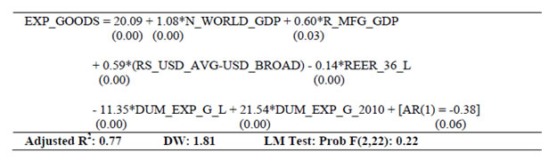 Variables: 5.2 Services Export Services Export = f (World GDP, Services GDP, Real Exchange Rate, Relative currency movement, Dummies) The specification for services export remains by and large the same as for the goods export equation apart from the fact that we use GDP in the services sector instead of manufacturing GDP. Estimated relationship of services exports is in line with merchandise in general. However, the impact of world GDP is lower for services exports as compared with merchandise exports, while domestic services GDP is far more important for services exports than manufacturing GDP is for merchandise exports. 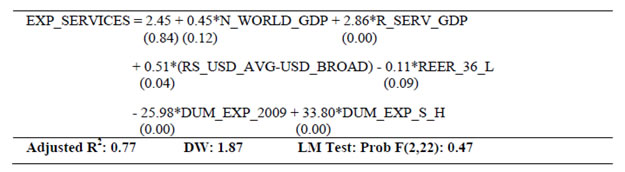 Variables: EXP_SERVICES: Growth of Services Exports (BoP basis in USD); N_WORLD_GDP: Growth of World Output (Current Dollars); R_SERV_GDP: Growth of GDP - Services Sector; RS_USD_AVG-USD_BROAD: Appreciation/depreciation in % terms of Indian currency over and above a broad set of other currencies (as included in US Broad Index) against the US Dollar (Nominal Appreciation (+)/Depreciation (-) of Rupee/Dollar Exchange Rate - Nominal Appreciation (+)/Depreciation (-) of other currencies (included in US Broad Index)/Dollar Exchange Rate), REER_36_L: Real Effective Exchange Rate (Trade Weighted, 36 Currencies); DUM_EXP_2009 puts 2009 = 1; else 0, DUM_EXP_S_H: 1980, 1998, 2004. 5.3 Goods Import Goods Import = f (Real GDP, World Crude Oil Prices, Real Exchange Rate, Relative currency movement, Dummies) Goods import is observed to be driven by GDP growth, world crude prices and exchange rate movement in real terms as also nominal appreciation/depreciation in relation to global currencies. Real exchange rate is impacting exports and imports on the expected lines. However, it is also evident that a higher pace of Rupee’s depreciation over other global currencies compresses imports during the year over and above the REER impact and vice versa. 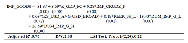 Variables: IMP_GOODS: Growth of Imports (BoP basis in USD); R_GDP_FC: Growth of GDP (Factor Cost, Constant Price); IMF_CRUDE_P: Global Crude Price; RS_USD_AVG-USD_BROAD: Appreciation/depreciation in % terms of Indian currency over and above a broad set of other currencies (as included in US Broad Index) against the US Dollar (Nominal Appreciation (+)/Depreciation (-) of Rupee/Dollar Exchange Rate - Nominal Appreciation (+)/Depreciation (-) of other currencies (included in US Broad Index)/Dollar Exchange Rate), REER_36_L: Real Effective Exchange Rate (Trade Weighted, 36 Currencies); DUM_IMP_G_L: 1981, 1983, 1984 and 1989 = 1; else 0;DUM_IMP_G_H: 1994, 2004. 5.4 Services Import Services Import = f (Non-agricultural GDP, Real Exchange Rate, Relative currency movement, Dummies) In services import, REER turns out to be statistically insignificant. Also, the impact of domestic economic activity is relatively muted as compared with merchandise imports. 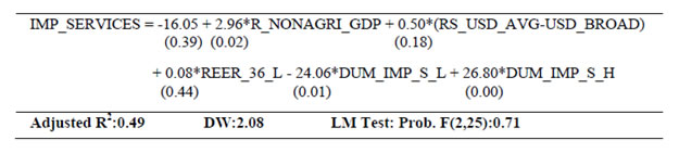 Variables: IMP_SERVICES: Growth of Services Imports (BoP basis in USD); R_NONAGRI_GDP: Growth of Non-agricultural GDP; RS_USD_AVG-USD_BROAD: Appreciation/depreciation in % terms of Indian currency over and above a broad set of other currencies (as included in US Broad Index) against the US Dollar (Nominal Appreciation (+)/Depreciation (-) of Rupee/Dollar Exchange Rate - Nominal Appreciation (+)/Depreciation (-) of other currencies (included in US Broad Index)/Dollar Exchange Rate), REER_36_L: Real Effective Exchange Rate (Trade Weighted, 36 Currencies); DUM_IMP_S_L: for the years 1985, 1996; DUM_IMP_S_H: for the years 1998, 2000, 2002, 2004. Capital Account The capital account is estimated by reclassifying individual items of net capital flows into debt and non-debt (equity) flows. Debt flows dominate total capital flows in India, until equity flows gain in prominence since 1994-95. The average share of equity flows at around 55 per cent exceeds that of debt flows in the total net flows since 2000. 5.5 Net Debt Flows Net Debt Flows = f(GDP growth, Interest differential, Relative currency movement, Inflation, Dummies) Capital regulations in debt flows are more prominent in India than in the case of equity flows. Yet it is observed that GDP growth facilitates higher demand for debt in India as it imparts greater confidence to overseas investors. The relative cost of borrowing for the domestic borrowers from foreign lenders measured as SBI advance rate net of one year LIBOR (USD), further adjusted for Rupee appreciation (+)/depreciation(-) during the year is also very close to statistical significance at 10 per cent level. The level of inflation is another important determinant of debt flows with higher inflation reducing the expected real cost of borrowing from domestic sources besides enhancing debt cost from abroad on deteriorating exchange rate expectations and vice versa. Therefore, it is also included as an explanatory variable, which is statistically significant. 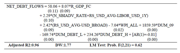 Variables: NET_DEBT_FLOWS: Growth of Net Debt Flows; R_GDP_FC: Growth of GDP (Factor Cost, Constant Price); N_SBIADV_RATE+RS_USD_AVG-LIBOR_USD_1Y: Interest rate differential adjusted for exchange rate appreciation/depreciation; RS_USD_AVG-USD_BROAD: Appreciation/depreciation in % terms of Indian currency over and above a broad set of other currencies (as included in US Broad Index) against the US Dollar (Nominal Appreciation (+)/Depreciation (-) of Rupee/Dollar Exchange Rate-Nominal Appreciation (+)/Depreciation (-) of other currencies (included in US Broad Index)/Dollar Exchange Rate); WPI_ALL: WPI Inflation; DUM09: Dummy for 2009; DUM_DEBT_L: Dummy for 1995, 1997, 2000, 2008; DUM_DEBT_H: Dummy for 1996. 5.6 Net Non-Debt (Equity) Flows Net Equity Flows = f (Growth differential, Capital flows to emerging countries, Stock returns, Relative currency movement, Own lag, Dummies) Higher growth differential (India’s GDP growth over world GDP growth) enhances country’s attractiveness to the global investors, domestic equity price indicates investment climate, and overall growth in net private flows to emerging market countries shows global risk appetite. These variables are incorporated in equity inflows equation in India along with relative currency movements of Rupee. It turns out that growth differential, equity price, overall equity flows to emerging markets as also the relative strength of Rupee as compared to other currencies attracts equity capital in a statistically significant manner. 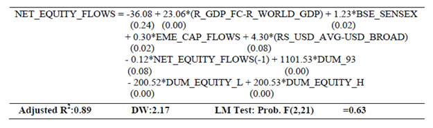 Variables: NET_EQUITY_FLOWS: Growth of Net Equity Flows; R_GDP_FC-R_WORLD_GDP: Growth of GDP (Factor Cost, Constant Price) minus World GDP Growth; BSE_SENSEX: Growth of Sensex; EME_CAP_FLOWS: Growth in net private financial flows to emerging market countries; RS_USD_AVG-USD_BROAD: Appreciation/depreciation in % terms of Indian currency over and above a broad set of other currencies (as included in US Broad Index) against the US Dollar (Nominal Appreciation (+)/ Depreciation (-) of Rupee/ Dollar Exchange Rate - Nominal Appreciation (+)/ Depreciation (-) of other currencies (included in US Broad Index)/ Dollar Exchange Rate); DUM_93: Dummy for 1993; DUM_EQUITY_L: years 1981,1990; DUM_EQUITY_H: years 1982, 1987. 5.7 Exchange Rate Exchange rate = f (Current account balance, Capital flows, Inflation, Dummies) Exchange Rate (Rupee/USD % changes) is regressed on current account balance to GDP ratio, capital account balance to GDP ratio and lagged inflation and they appear with expected signs and significance. 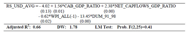 Variables: RS_USD_AVG: Nominal Appreciation (+)/Depreciation(-) of Rupee/Dollar Exchange Rate; CAB_GDP_RATIO: Ratio of Current Account Balance to GDP; NET_CAPFLOWS_GDP_RATIO: Ratio of Capital Flows to GDP; WPI_ALL(-1): One year lag of WPI Inflation; DUM91_98: Dummy for the years 1991 and 1998. Section V: Concluding Observations Econometric models have emerged as an effective tool for central banks for medium to longer term economic forecasts and policy analysis. Central banks spend considerable resources for model development and addressing its gaps for its other practical use. Central banks rely not just on one model but a suite of models, each of them having their own pros and cons, but when combined, imparts greater confidence. This paper estimates a set of equations establishing linkages within and across various sectors of the Indian economy for enabling an econometric model for India. Accordingly, the macro-economy consists of five sectors, namely the real, prices, monetary, fiscal and external sector. Equations within each of them are developed at a disaggregated level to work out appropriate mapping of relations for further use. All estimations are made over the sample period 1980-81 to 2012-13 with annual data. The equations have been estimated by ordinary least squares with appropriate dummies. The forecasts of the macro-aggregates can technically be obtained, although may not be desirable owing to the fact that parameters are averages over a very long period of time with many structural breaks. This can nevertheless offer insights for extending these relations in the context of an econometric model to address important issues faced by monetary policy in India. The set of equations together portrays a transmission network from monetary policy instruments/rates to money market rate to a broader spectrum of deposit and lending rates. Through deposit and credit aggregates, it also shows up on the broader real economy. Fiscal condition impacts lending rates, and higher government borrowings crowds out private sector borrowings. The impact of credit cost on private investments is prominent. The monetary policy variables like money growth and interest rate affect non-food manufactured product inflation. Global integration and exchange rates have notable impact on several components of WPI inflation. Exchange rate affects prices directly through imported goods and has an indirect impact through net exports and real GDP. The growth of real GDP and prices impact many other variables in the fiscal and external sectors. The revenue growth of the government as also government’s capital expenditure shows higher pro-cyclicality. Revenue expenditure on the other hand is relatively sticky, while government’s ability to spend depends on its cost of borrowings to a large extent. Within the external sector, India’s services sector output growth shows a far greater influence on India’s services exports as compared with a similar impact of the manufacturing growth on the merchandise exports. With respect to the global income elasticity of India’s export, services exports exhibit relative resilience to the global growth cycle as opposed to merchandise exports showing large movements in response to the same. India’s imports of goods and services also show high elasticity in response of domestic activities. The impact of real exchange rates on both exports and imports are relatively small. Rather, the relative changes in nominal Rupee movements vis-a-vis other currencies appear to have an important role. @ Rajib Das is Director, Binod B. Bhoi and Pankaj Kumar are Assistant Advisers, and Krittika Banerjee is Research Officer in the Department of Economic and Policy Research. 1The authors acknowledge the encouragement of Shri Deepak Mohanty, Executive Director and Shri Amitava Sardar, Adviser in preparation of this paper, but take full responsibility for any errors and omissions. References
Sector 1: Monetary Sector Money supply (Components side)
Money supply (Sources side)
Interest Rates
Identities
Sector 2: Prices Sector WPI Components
Identities (Weighted Sum)
Sector 3: Real Sector Demand Side Consumption
Investment
Identities
Supply Side Stochastic equations:
Identities:
Sector 4: Fiscal Sector Receipts
Expenditure
Identity
Sector 5: External Sector Current Account
Capital Account
Exchange Rate
Identities
Annex 3: Plot of CUSUM and CUSUM of Squared Errors from Recursive Regression 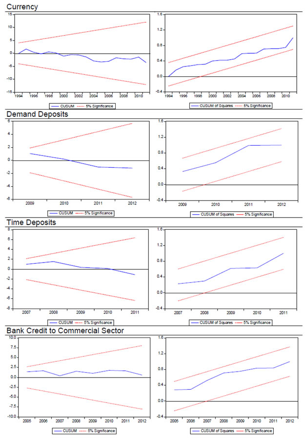 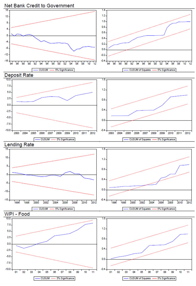 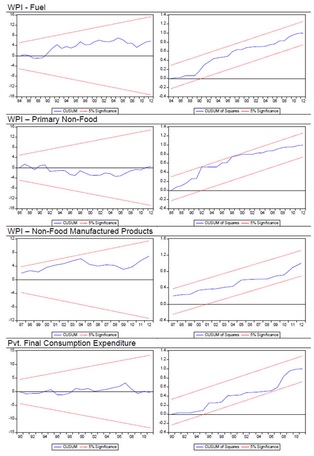 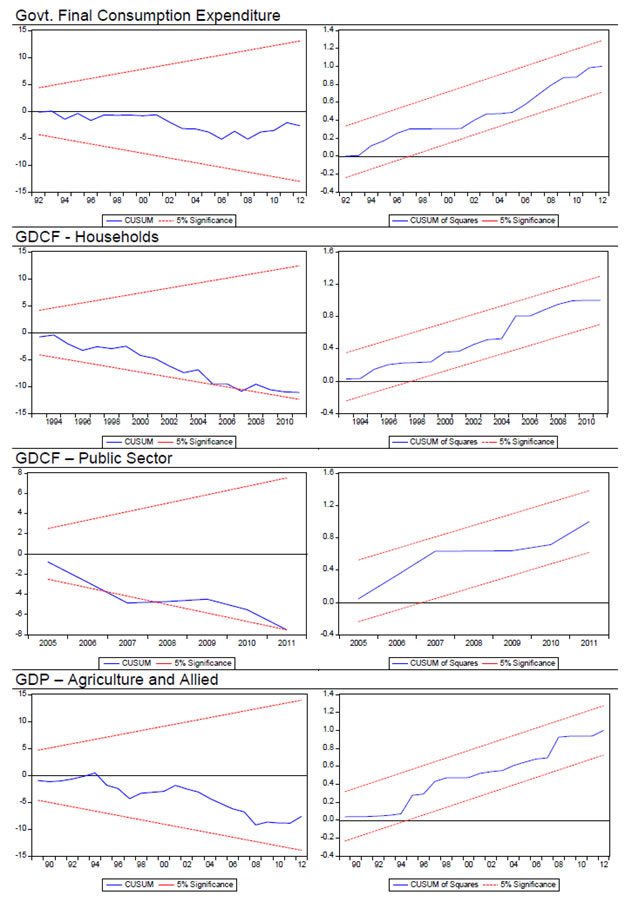 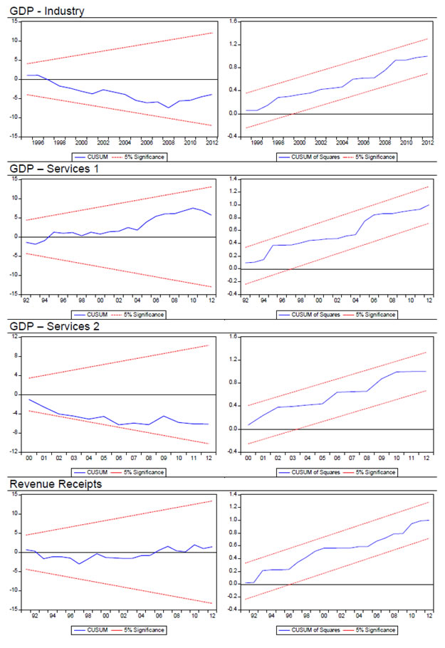 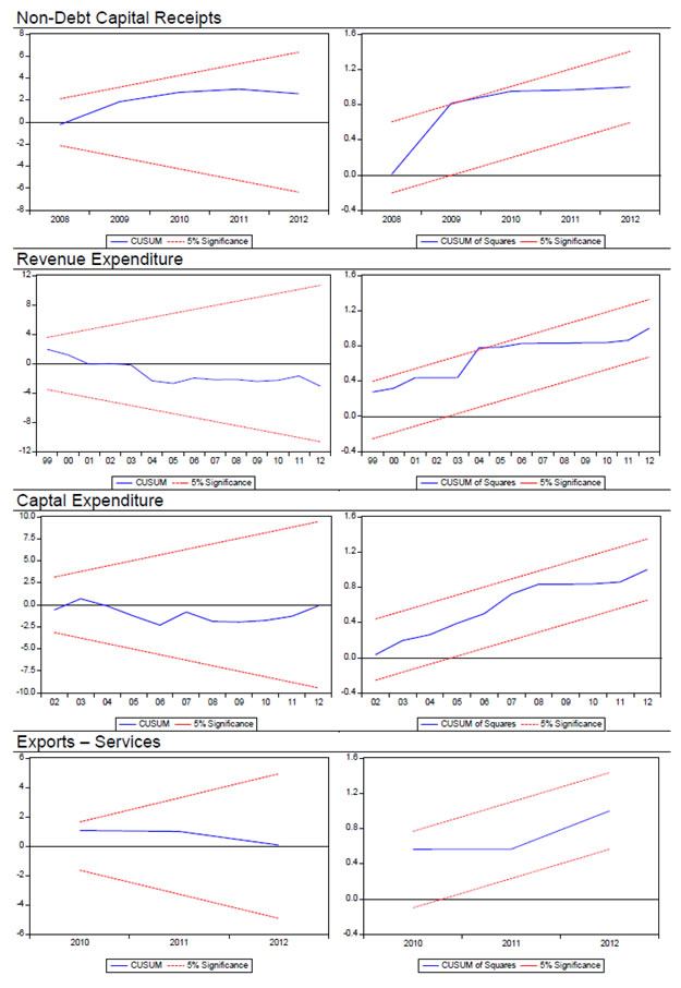 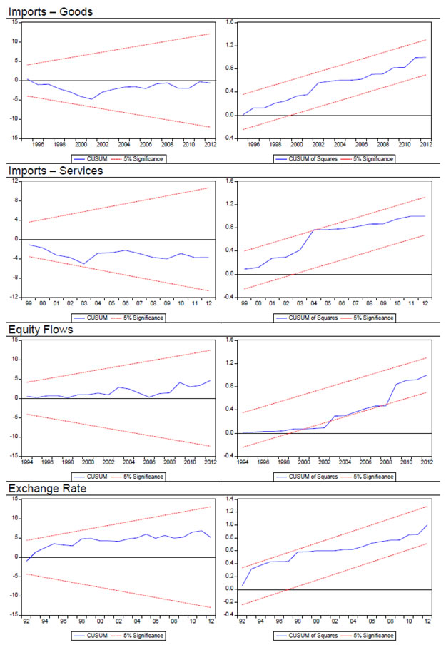 |

Share this page:


Install the RBI mobile application and get quick access to the latest news!
Scan the QR code to install our app


Page Last Updated on:


