 IST,
IST,


RBI WPS (DEPR): 06/2024: Price Dynamics and Value Chain of Fruits in India: A Study of Grapes, Bananas and Mangoes
|
Price Dynamics and Value Chain of Fruits in India: A Study of Grapes, Bananas and Mangoes1 Raya Das, Ranjana Roy, Sanchit Gupta, Sanjib Bordoloi, Rishabh Kumar, Renjith Mohan and Ashok Gulati1 Abstract The paper analyses the determinants of prices of select fruits – grapes, bananas, and mangoes – in India following a monthly balance sheet approach based on primary survey-based information and secondary data. The perishable nature of fruits and their inherent seasonality underscores the importance of evaluating supply and demand dynamics to analyse and forecast fruits prices. The paper also assesses the value chains in these fruits using insights from interactions with farmers, traders, and processors. The paper estimates farmers’ share in the consumer rupee which works out to 31 per cent for bananas, 35 per cent for grapes and 43 per cent for mangoes in the domestic value chain. In the export value chain, while the share is higher for mangoes, it is lower in case of grapes, although the realised price is higher than the domestic value chain. The empirical analysis based on Autoregressive Distributed Lag (ARDL) models suggests a long-run inverse relationship between availability/ availability-usage ratio and prices of the selected fruits. The paper forecasts inflation over a 12-month horizon using univariate and multivariate time-series models integrating the balance sheet variable. The forecast evaluation suggests a generally superior performance of Seasonal Autoregressive Integrated Moving Average with Exogenous Variable (SARIMAX) models over different horizons, underscoring the importance of the balance sheet variable for understanding the price dynamics of selected fruits. JEL Classification: E31, E37, E52, Q11, Q13 Key Words: Balance sheet, grapes, mango, banana, forecast, inflation, value-chain, SARIMAX, survey, farmers Price Dynamics and Value Chain of Fruits in India: A Study of Grapes, Bananas and Mangoes Introduction The horticulture sector in India has witnessed remarkable growth in recent years with a substantial share of 36 per cent in the gross value of output (GVO) of agriculture, with fruits constituting 37 per cent of horticulture output as of 2022-232. The surge in horticulture production has been driven by the expansion of area from 23.2 million hectare (Mha) in 2011-12 to 28.4 Mha in 2022-23. In the case of fruits, the increase in production is also attributed to the rise in yield from 11.4 metric tonne (MT) per hectare in 2011-12 to 15.7 MT in 2022-23. Accordingly, the same period witnessed an increase in overall fruits production from 76.4 million metric tonne (MMT) to 110.2 MMT. The United Nations General Assembly (UNGA) declared 2021 as the International year of fruits and vegetables to increase awareness about nutritional benefits of fruits and vegetables, to promote environmental sustainability and to secure livelihood of farmers. Nevertheless, fruits and vegetables marketing, particularly in developing countries, faces multiple challenges of transport cost, seasonal glut, supply shocks, quality checks, labour intensive production system and post-harvest losses impacting inflation and volatility in their prices (FAO, 2020). Fruits are high-value agriculture crops and therefore volatility in their prices impacts the purchasing power of households and hence the consumption pattern. In India, ebbs and surges in inflation are often driven by volatile food prices. Such swings in the inflation trajectory pose challenges for the conduct of forward-looking monetary policy, as food prices have the potential to impact inflationary expectations. In view of the overlapping supply shocks since the onset of the pandemic, the large fluctuations seen in food prices calls for a deeper understanding of food price dynamics and value-chains of agricultural commodities in India. In India, supply shocks to agriculture production result in high inflation volatility due to high share of food and beverages in the Consumer Price Index (CPI) basket (weight of 45.9 per cent in the CPI-combined at 2012 base). The three fruits selected for this study - grapes, banana, and mango - have around 36 per cent share in the CPI-fruits basket3 and contribute significantly to the inflation volatility of the group. Rainfall, input prices, rural wages, supply-chain measures and government policies influence agricultural commodity price inflation (Gulati & Saini, 2013). Nair & Eapen (2015) analysed various factors impacting agriculture commodities inflation between 2009 and 2013 and found that the increasing cost of cultivation is the major factor driving fruits inflation. On the demand side, while the consumption pattern has shifted from cereals to protein-rich food, the pace of transition to nutrient rich fruits, however, has been slow and differed across regions (Agrawal & Kumaraswamy, 2014; Tak et al., 2019). This study also found that the share of non-consumption of fruits in the eastern states is the highest (30 per cent) followed by the northern states (20 per cent) as of 2011-12 recall period. Against the backdrop of changing consumption and production pattern and price volatility, this paper analyses the price dynamics and determinants of fruits prices following a comprehensive balance-sheet approach designed to capture the interplay of demand and supply side factors. It uses the constructed availability-to-usage (AVU) variable from the monthly balance sheet as one of the key explanatory factors and employs time series models to generate short-term inflation forecasts. As the supply chain plays an important role in stabilising prices, the study also traces value-chain efficiency and its impact on the farmers’ share in the consumer rupee for fruits and suggests interventions for better supply-chain management. The paper constructs balance sheets of the select fruits using secondary data sources and market intelligence from primary surveys. The broad objectives of the study are:
The empirical findings suggest that the monthly availability or availability-usage ratio negatively impact retail prices of the selected fruits. Input prices (proxied by pesticides, agrochemicals) also influence fruits price dynamics. The study also assesses the value chain and its impact on fruits price dynamics to suggest necessary policy interventions. Based on survey data, farmers’ share in the retail prices of these fruits is estimated in the range of around 30 to 43 per cent, with the shares varying across marketing channels. The rest of the paper is organised into nine sections. Section II provides a broad overview of grapes, banana, and mango. Section III examines the price dynamics of the fruits along with their seasonality. Section IV reviews the literature covering the role of supply and demand factors to trace the key determinants of fruits prices in India for their use in the econometric models. Section V maps the value chain of grapes, banana and mango, and estimates farmers’ share in the consumer rupee to assess the efficiency of value-chain. It also provides a brief profile of market intelligence and key informants of primary field surveys. Section VI elaborates the methodological framework for construction of the monthly balance sheets for understanding fruits price dynamics. Section VII specifies the model and provides the empirical results highlighting the important structural drivers of fruits prices. Section VIII generates inflation forecasts of the selected fruits for a horizon of up to 12 months and evaluates the forecasting performance of alternative econometric models. Section IX draws major conclusions from the study and provides policy suggestions aimed at improving the supply chain for taming fruits price inflation. II. Commodity Profile India’s varied agro-climatic regions and tropical location make it possible to grow large varieties of fresh fruits. The country ranks second in fruits and vegetables production in the world, after China. According to the Food and Agriculture Organisation (FAO, 2022), India ranks first in the production of banana (with a share of 26 per cent) and mango, including mangosteens and guavas (44 per cent), and second in fresh/ table grapes (12 per cent). The huge production base offers India incredible opportunities for export. During 2022-23, India exported fresh fruits and vegetables worth US$ 1,789 million, out of which fruits accounted for US$ 863 million. II.1. Grapes Production Global grapes production is divided into pressed grapes (37.3 MMT in 2022) and unpressed grapes (35.5 MMT)4. According to FAO, China is the largest producer of total grapes (fresh/table, raisin, and wine) at 12.6 MMT followed by Italy (8.4 MMT), France (6.2 MMT), Spain (5.9 MMT), and the US (5.3 MMT). India ranks seventh at 3.4 MMT in 2022, accounting for 4.5 per cent of total global grapes production (Chart 1). As per National Horticulture Board (NHB), India's production of total grapes has increased from 2.2 MMT in 2011-12 to 3.7 MMT in 2022-23. This is driven by both higher area and yield (Chart 2). Global table grapes production is about 31.5 MMT (42.0 per cent of total grape production) and India is the second largest producer of table grapes after China (International Organisation of Wine and Vine (OIV) Report, 2022). In contrast to the expansive growth of the winery sector in the EU and the US as indicated by FAO (2022), India has emerged as a prominent producer of table grapes – those intended for direct consumption. Since the 1960s, with the introduction of seedless varieties, grape production - Viticulture - commenced in Maharashtra which accounts for 78 per cent of total grapes production in the country, followed by Karnataka at 18 per cent in triennium ending (TE) 2022-23 (MoA&FW, 2023) (Chart 3). Of the total grapes production in the country, fresh grapes constitute 77 per cent followed by raisin (20 per cent), wine grapes (2 per cent), and juice and concentrates (1 per cent) (Agricultural and Processed Food Products Export Development Authority (APEDA), 2021). Grape production is regionally concentrated in tropical peninsular India. The major growing districts are Nashik, Sangli, Solapur, Pune, Satara, Latur and Osmanabad in Maharashtra; and Bijapur, Bagalkot, Belgaum and Gulberga in Karnataka. Furthermore, a marginal grape cultivation presence is noted in select sub-tropical regions, including Bhatinda, Gurdaspur and Ludhiana districts of Punjab and Hissar and Jind districts of Haryana. However, the annual growth rate of grapes production has declined in Maharashtra from 8 per cent in the triennium ending (TE) 2014-15 to 2 per cent in TE 2022-23. In contrast, the share of Karnataka in terms of area and production have been increasing over the years. The share of grapes for wine processing and raisin production is higher in Karnataka, whereas Maharashtra is the epicentre of fresh grapes production. In terms of variety, Nashik cluster is the major producer of Thompson seedless (T. seedless) variety which comprises 55 per cent of total table grapes production (Chart 4). In sub-tropical region, due to short span of growth time, Perlette variety is grown at a meagre level. The regional demand in Punjab and Haryana is also higher than the other states, hence this variety caters to the demand during the pre-monsoon months of May-June. Bangalore blue, Anab-e-Sahi, Muscat and Bhokri are the major varieties in Karnataka. Karnataka region has two harvest seasons, one is during January-March and the other is during September-December. In the main cluster of grape production i.e., Maharashtra, harvest of grapes has single window between January-May. India is also the third largest consumer of table grapes followed by China and Turkey as per the International Organisation of Vine and Wine (OIV, 2022). Per capita consumption of grapes, however, has rural-urban disparities – monthly consumption was 38 grams in rural area, and 84 grams in urban area in 2011-12. Even though market intelligence indicates higher quantity of grapes consumption (150-160 grams per capita in rural-urban combined area), the consumption figure of National Sample Survey (NSS) 2011-125 has been used in this study owing to the large-scale sample coverage of the survey. Around 7 per cent of rural households and 13 per cent of urban households reported grapes consumption during that year. Regional patterns shows that eastern states have very low consumption of grapes, whereas consumption is much higher in southern, western and north-western states. In rural areas, consumption of grapes is highest in Kerala (100 grams per capita per month) and in urban areas, Delhi, Mumbai and Hyderabad are the major consumption centres. As per class-wise monthly per capita consumption expenditure (MPCE) decile, top-most class consumes 138 grams per capita per month in rural area, as against 25 grams in the sixth decile class. On the other hand, in urban areas per capita consumption is 246 grams per capita per month in top-most class in comparison to 66 grams for the middle MPCE class (NSO, 2013). External Trade World fresh grape trade was 5.2 MMT in 2022 with Chile being the largest exporter (despite being 8th largest producer in TE 2021-22) followed by Peru and Italy. India imports grapes mainly from China, while its primary export destinations are Netherlands and Bangladesh (Chart 5). Seccia et al., (2015) highlighted that India is emerging as a major competitor in the northern hemisphere along with China, Egypt, Mexico and Turkey. Unit value of export (UVE) of India, however, has generally been lower than Chile due to production shortage, and high shipping cost (Annex-Chart A1). Nonetheless, India’s export value rose by more than 4 times from Rs.5.1 billion to Rs.23.0 billion in the last decade. Similarly, the overall grape imports also increased in India, from around 4 thousand tonnes in 2011-12 to 12 thousand tonnes in 2022-23, although there was a dip in the pandemic year. After 2015, however, imports of coloured varieties of grapes have shifted from USA to China. Export quantity has been increasing due to betterment in EurepGAP6 and increase in production (Phadke et al., 2022). For the first time, after EU consignment rejection in 2021, export quantity towards Bangladesh overtook exports to EU. However, Bangladesh has imposed high import duty for Indian grapes (25 per cent) since January 2023 (Market intelligence, APEDA). Following the peak period of production (February-March), India exports the maximum quantity of grapes in March, whereas the peak of imports happens in October. Demand generally increases during September-October due to the festive season in India. However, during the lean season, as domestic production does not fully cater to the domestic demand, the shortfall is met through imports (Chart 6). II.1. Banana Production Bananas are predominantly produced in Latin America, Asia and Africa. In 2022, India was the largest producer of banana (34.5 MMT or 26.3 per cent of global production), followed by China, Indonesia, Brazil, Ecuador and Philippines (Chart 7). Production in India mostly caters to the domestic market. In India, the most popular commercial Cavendish cultivar variety of banana is grown in states of Maharashtra, Gujarat, Bihar, West Bengal, Tamil Nadu, Karnataka and Andhra Pradesh. Other varieties include Robusta, Rashthali, Poovan, Nendran, Red Banana, Ney Poovan, Virupakashi, Pachanadan, Monthan, Karpuravalli and Safed Velchi Musa, which are mostly produced and consumed locally. Banana is the second most important fruit in India with around 13 per cent of total fruits area allocated to the production of banana. Of the total value of fruits output, banana is the second largest contributor (24 per cent) after mango (29 per cent). The production of banana has increased from 26.5 MMT in 2012-13 to 36.6 MMT in 2022-23, while the area under banana has increased from 0.78 Mha to 0.99 Mha over the same period (Chart 8). The major banana producing states include Andhra Pradesh (with a share of 18.1 per cent) followed by Maharashtra, Tamil Nadu, Gujarat, Uttar Pradesh, Karnataka and Madhya Pradesh, together contributing around 80 per cent of the total production in TE 2022-23 (Chart 9). Banana is a perennial crop, available throughout the year. In states like Gujarat, Uttar Pradesh, Bihar and Jharkhand, the peak season of banana harvest falls during September-November, whereas in Maharashtra, the peak harvest months are April-May. In South Indian states, planting can be done at any time except for the peak summer months. External Trade World trade in banana has expanded in the recent years with an estimated exports of 21 MMT in TE 2021-22. The leading exporting regions of banana are Latin America and Caribbean contributing 75 per cent of world exports, followed by Asia (21 per cent) and Africa (3 per cent). The major banana exporting countries are Ecuador, Philippines, Costa Rica, Guatemala, Colombia, and Dominican Republic. The leading importing countries are European Union (with a share of 26.3 per cent in total imports), USA (21.3 per cent), China (10.6 per cent), Russian Federation (7.4 per cent) and Japan (5.7 per cent). According to FAO, banana shipment has contracted from Asia in the post pandemic period. Philippines being the major exporter from Asia (60 per cent of Asian exports) suffered heavily due to the spread of Tropical Race 4 (TR4) banana disease in 2020-21. The exports of banana from India have increased from 35 thousand MT in 2013-14 to 376 thousand MT in 2022-23 (Chart 10). However, India’s exports constitute less than 2 per cent of world exports as India is also the largest consumer of banana (Chart 11). India’s domestic farmgate banana prices doubled from Rs.14-15 per kg during 2021-22 to Rs.27-28 per kg during 2022-23 (Market Intelligence, 2023), contributing to a decline in the export shipment in 2022-23. II.1. Mango Production India is the largest producer of mango globally (Chart 12)7. In TE 2022, India produced 25.3 MMT which accounts for 44.6 per cent of the total global mango production (FAOSTAT, 2022). Other top producing countries are China (3.8 MMT), Indonesia (3.8 MMT), Pakistan (2.6 MMT), Mexico (2.4 MMT) and Brazil (2.1 MMT). India is also the largest consumer of mango in the world. The yield of mango in India stood at 9.5 tonnes/ha8 in 2021, at par with the world average (FAOSTAT, 2022). However, the yield is higher in China and in Indonesia at 10.2 tonnes/ha and 13.4 tonnes/ha, respectively. Mango production in India has increased at a compound annual growth rate (CAGR) of 2 per cent from 16.2 MMT in 2011-12 to 20.9 MMT in 2022-23. The area under mango cultivation, however, has declined to 23.4 lakh hectares (Lha) in TE 2022-23 from 24.6 Lha in TE 2013-14 (NHB, 2022). The increase in the production was thus driven by increase in domestic yield from 6.8 tonnes/ha in 2011-12 to 8.9 tonnes/ha in 2022-23 (Chart 13). Andhra Pradesh and Uttar Pradesh dominate mango acreage in India with a share of 17 per cent and 12 per cent, respectively. They also have a dominant share in total production at around 23 per cent each (Chart 14). Mango cultivated in Uttar Pradesh, Andhra Pradesh, Bihar, Karnataka, Gujarat, Tamil Nadu and Telangana comprise 75 per cent of total production and have higher degree of commercialisation compared to other mango producing states. External Trade Some key globally traded mango varieties are Tommy Atkins (Latin America), Kent (Florida), Keitt (Florida), Palmer (Israel), Amélie (Africa) and Irwin (Latin America). In 2021, Mexico had the largest share in global exports at 16 per cent followed by Thailand with 14 per cent (Chart 15). India is a net mango exporting country with a share of 6 per cent in global exports in 2021. Alphonso (Maharashtra), Kesar (Gujarat), and Banganpalli (Andhra Pradesh and Tamil Nadu) are the leading export varieties from India. Notwithstanding the reduced acreage, Maharashtra continues to play a vital role in India’s Alphonso exports. Other major exporting states are Gujarat, Tamil Nadu, West Bengal, Karnataka and Andhra Pradesh. India’s exports remain low (0.8 per cent of its total production in 2021-22) despite India being a top producer in the world as a large portion of total production is consumed domestically (DGFT, 2023) (Chart 16). Mango exports are primarily of three forms: (i) fresh mango, (ii) mango pulp, and (iii) mango slice. Mango pulp comprises the major share (78 per cent) of mango exports from India as per TE 2022-23, followed by fresh mango (17 per cent) and mango slices (5 per cent). This has changed only slightly from TE 2013-14 when the shares of mango pulp, fresh mango and mango slices were at 73 per cent, 25 per cent and 2 per cent, respectively (DGFT, 2023). The export volume of all three mango forms has declined in the last decade, with mango pulp recording a steady decline with little to no recovery. Major export destinations for fresh mango are UAE, the UK, the US, Oman, Qatar, and Nepal. Mango pulp is exported mainly to Saudi Arabia, Yemen Republic, Netherlands, Kuwait, the UK, and the US. Although UAE has remained the top destination for fresh mango exports, its share in India’s total mango exports has seen a decline from 54.3 per cent in 2015-16 to 46.4 per cent in 2021-22 (APEDA, 2022). On the other hand, share of exports to Bangladesh and Oman increased considerably from 0.9 per cent to 5.6 per cent, and from 2.5 per cent to 6.6 per cent, respectively. III. Price Dynamics of Fruits Fruits, similar to other horticulture crops, witnessed price volatility due to weather vagaries, rising cost of cultivation, pandemic shock and disruption in supply chains. Fruit items constitute only 6.3 per cent of CPI-Food and beverages weights, within which banana comprises the largest share (19.4 per cent), followed by apple (16.3 per cent), mango (11.1 per cent), coconut (9.1 per cent) and grapes (5.3 per cent). Although fruits make up a modest portion of the CPI basket, their prices exhibit noteworthy volatility (Chart 17). During January 2023 to December 2023, fruits inflation contributed about 1-9 per cent to overall food and beverages inflation (Chart 18). The climatic challenges often lead to supply constraints, exerting pressure on fruit prices. During the summer months, the contribution of mango in CPI fruits inflation is the maximum, reflecting its seasonality as well as its higher demand during the beginning of the harvest season. In 2022, mango prices increased sharply due to low harvest; but moderated in 2023 with normal production of the crop. The contribution of banana in CPI fruits inflation remained elevated throughout 2023 while apple was a major contributor from June 2023 to December 2023 (Chart 19). III.1. Grapes Grapes experienced high inflation in May 2014, May 2018 and August 2021 at 22.1 per cent, 26.2 per cent and 17.2 per cent, respectively. Generally, price rise from June onwards is due to seasonality, as it is the end of fresh grapes harvest season and the reduction in market arrival cannot cater to the demand of summer months. During the summer months, brix (a measure of sugar content) value of grapes also increases, hence market demand also rises. Crop calendar of grapes indicates peak arrivals during the months of February-March (Table 1), when 75 per cent of produce comes to the market (as per market sources). In Karnataka, coloured varieties are grown, particularly Bangalore blue, which is more expensive than T. seedless, resulting in higher prices during June-July. The ratio of monthly retail price of grapes to all India monthly average retail price of grapes as of TE 2021-22 has been used to gauge seasonality of retail prices. The price is the lowest during February-March, the peak harvest months of the produce (Chart 20). Average price during TE 2021-22 indicates that prices dropped from Rs.109 per kg in January to Rs.83 per kg in March. Retail prices and market arrivals show distinct inverse relationship, and the seasonality is at its peak in August, with three years average price of Rs.155 per kg for Thompson Seedless variety. As the market presence is meagre and the import quantity is more during July-November, the retail price of grapes is higher due to both supply shortage and costlier import. Also Red globe is the major grape variety for import which is more expensive than Thompson seedless or its cultivars (major grape variety in domestic market). III.2. Banana Banana retail price inflation spiked to a high of 18 per cent during September-December 2013 due to monsoon deficiency and decrease in area under cultivation (Chart 21). The area under banana had dropped from 0.83 Mha in 2010-11 to 0.80 Mha in 2011-12, and further to 0.78 Mha in 2012-13. As banana cultivation requires higher water supply, depleted water level forces banana growers to move to other crops. Moreover, banana crop is often plagued by pest attack that hampers harvest severely. For instance, a widespread attack of ‘banana skipper’ pest in Karnataka in 2015-16 resulted in almost 30 per cent weight loss (Prabhu, 2015). Regular monitoring for infestation and applying agro-chemical sprays inflate the cost of cultivation. In 2017-18, there was an outbreak of Panama disease/ TR4 which infected more than 10,000 ha of plantation and impacted retail inflation of banana. In March 2023, a steep rise in banana prices was observed in the major urban pockets. According to traders, this spike in prices was attributed to rising transport and storage cost as well as increase in the gap between demand and supply, due to heavy rains in states like Gujarat, Maharashtra, and Andhra Pradesh. III.3. Mango Mango being a summer fruit, the CPI for mango is available seasonally from April to August every year. Before 2018-19, however, the data was released for every month. Therefore, price behavior in these five months of mango production in India is analysed in this section. A plot of CPI and Wholesale Price Index (WPI) inflation of mango depicts wide gaps, which possibly can be explained either through inefficient value chain, high retailer margins or differences in the way the data are collated. There are periods when both the indices move in opposite directions, which could be due to the difference in varieties of mango at the time of collating price quotations for constructing these indices (Chart 22). Nonetheless, the correlation between CPI and WPI inflation in mango is 0.69. Every year, March sees the beginning of arrivals of the produce which peaks in June when mango arrivals from Uttar Pradesh are at their peak and then falls in August. The seasonality in retail prices along with the mandi arrivals pattern of mango in India indicates an inverse relationship between them (Chart 23). The mango arrivals overlap for different varieties in May and June as the north Indian varieties like dusheri, chausa arrives in the market with other varieties like Alphonso, Kesar, etc. There are high price variations variety-wise in mango and the difference between retail and wholesale prices of different varieties gives an indication of retail margins. The concentration of mango production and the logistics requirement for inter-state trade plays a role in the large price variation of the same produce at different geographical locations (different consumption centres). Though the value chain of mango involves many participants, and the costs of transportation and quality maintenance are high as well, we find that on an average, alphonso variety has a 62 per cent retail margin during April-August, while chausa, dusheri and kesar have 52 per cent, 44 per cent and 45 per cent margins, respectively. IV. Review of Literature With the change in dietary pattern alongside rising income, fruit sector in India has immense capacity to cater to this demand, augment farmers’ income and increase foreign exchange reserves. Studies have identified fruits and vegetables as dominant indicators explaining food inflation in India (Mishra and Roy, 2012). Inflation in India in food commodities particularly for pulses, milk, vegetables and fruits is due to shift in dietary pattern, trade policy and increase in rural wages (Ball et al., 2016). Bhattacharya and Sengupta (2015) argued that during 2006-13, supply of fruits generally exceeded domestic demand, resulting in moderate inflation in the sector. The production of fruits is determined by area under cultivation, environmental condition of growth including days of sunshine, rainfall, cyclones, and pest attacks. Temperature impacts production of fruits; heatwaves, particularly during the fruiting stage, leads to loss in harvest. Fruits production is also influenced by soil degradation, water shortages, and diseases. Climate change, temperature anomaly and erratic rainfall impact horticulture production, distorting crop cycle and production (Dutta, 2013). The cost of production has been escalating since the 1990s due to rise in agricultural wages and input costs (Narayanmoorthy, 2013). Increasing pest attack in tropical fruits has increased pesticide usage in India, with highest usage recorded in Punjab (0.74 kg per ha. in 2016-17), inflating the cost of cultivation. Moreover, in tropical fruits use of chemicals (growth regulators) for better growth of produce is higher. Further, post-harvest loss impacts domestic availability which often generates supply shortages leading to inflationary pressures. The post-harvest losses occur due to inefficient infrastructural facilities in the supply chain including inadequate number of cold storages, and phytosanitary measures, across different fruit crops, leading to widening gap between production and availability (Bairwa et al., 2012). The prices of fruits are also related to the post-harvest qualitative loss. Due to improper handling of banana, lack of proper transport facilities and storage environment, post-harvest loss is high in the commodity (Mohapatra et al., 2010). However, post-harvest loss for mango has declined from 12.7 per cent in 2005-07 to 9.2 percent in 2015-16. The estimates of post-harvest loss for grapes in Karnataka and Andhra Pradesh were 21.3 per cent in 2011 (IIHR, 2014). According to the CIPHET-ICAR (2015) study, at all India level, the total loss of grapes rose to 8.6 per cent in 2015-16 from 5 per cent in 2005-06. The trend was similar for banana, with loss increasing from 6.6 per cent to 7.8 per cent during the same period. More recent study by NABCONS (2022) shows, the total loss for grapes, banana, and mango at 7.2 per cent, 7.6 per cent, and 8.5 per cent respectively. On the demand side, the increase in per capita income has escalated the consumption of high value income elastic commodities including fruits (Rao et al., 2006). With economic growth and urbanisation, global trade in fruits and vegetables is growing rapidly. However, the tariff rates are not uniform across importing countries and higher import barrier results in inflation in the domestic market (Aksoy and Beghin, 2004). On the other hand, increase in demand for Indian fruits in the global market puts price pressure in the years of shortages in market availability. V. Value Chain Analysis of Fruits Institutional arrangements of value chain of fruits are quite different from cereals and vegetables like potato and onion due to their higher perishability and marketing risks. Amongst fruits, post-harvest loss is the highest for mango (9.2 per cent), followed by grapes (8.6 per cent) and banana (7.8 per cent). In order to strengthen fruit sector and increase its global competitiveness, the MoA&FW, GoI initiated a Cluster Development Program (CDP) implemented by NHB, to identify regional centres of fruit crops. The objective is to promote holistic development of value-chain from monitoring cultivation practices to technological change in supply chain for fostering climate resilient and economically remunerative horticulture sector. Out of the 12 clusters, two clusters are for banana in Theni, Tamil Nadu and Anantpur, Andhra Pradesh; three clusters for mango at Mahbubnagar in Telangana, Lucknow in Uttar Pradesh and Kutch in Gujarat; and one cluster for grapes at Nashik, Maharashtra. Against this backdrop, this section analyses the value chain of these three commodities based on global competitiveness, farmers’ share in consumer rupee and sustainability. The purpose of value chain analysis (VCA) is to map all economic players in the market of the specific commodity which impact the price of the final produce (FAO, 2014). For this purpose, the study uses both secondary sources and primary field surveys data collated by non-parametric purposive method of sampling through personal interviews of key informants, focused group discussions, and telephonic survey to gather market intelligence. The details of data sources are provided in Annex Table A4. The time period of the study is April 2012-December 2022 for grapes, July 2012-June 2022 for banana, and January 2011- August 2022 for mango depending on seasonality of the crop and data availability. V.1. Grapes Grapes in fresh and processed form are one of the most traded fruits in the world. As fresh fruit grape is very delicate, it is vulnerable to harvest and post-harvest loss, particularly quantity loss in retail chain due to shattering and discolouration (Nanda et al., 2012; Jha et al., 2015). Grape production is concentrated in Maharashtra and Karnataka and the domestic demand is mostly catered from the Nashik belt of Maharsahtra which has high share in total fresh grapes production (Chart 24)9. Hence, a forward and backward linkage analysis of value chain of the region has been done to understand the efficiency of the grape value-chain and its impact on the price dynamics. The black soil with low pH and climatic condition permits growth of grapes in the region. The average landholding under grapes in Maharashtra is 1-2 acres (NSO, 2019); hence, mostly growers are small producers. Technological change in distribution is nascent in developing countries including India. To trace the efficiency of value-chain, focused group discussions (FGDs) were conducted with domestic traders , grower exporters , farmers , merchant traders from Maharashtra and detailed personal interviews of farmers , domestic traders , exporters , cold storage owners, APMCs (Vashi, Pimpalgaon APMC, private fruit mandi), transport association for perishable commodities, raisin processing unit owner, and farmer producer company. The following analysis of value chain components is based on the information from field surveys and other secondary sources. The grape value chain of Nashik region is mapped in Chart 25. In the backward linkage of value-chain, farmers generally purchase rootstock from nurseries and plant it after establishing trellis for growth. Grape is a standing crop and after plantation it takes two years for first budding, and the lifespan of plant is 7-8 years. Pruning10 of grape plants happens in September-October months and within 90-120 days grapes get ready for harvest. Timing of pruning is critical; ideally farmers try to do pruning in early October as price stays high during the start of the harvest season (January). Due to rainfall, the pruning time was delayed by a month for three consecutive years 2018-2021, resulting in shortage of arrival in January. Early harvest of grapes occurs during November in Satana taluka in Nashik district, and even though the quantity is less, it caters to the festive demand along with imported grapes. However, late monsoon rainfall affects grape harvest during this period. Farmer interviews highlighted that climate change related weather vagaries are impacting the grape production cycle. Low temperature, lower daylight, hailstorms, and unseasonal rain in January month deteriorate the quality and quantity of grape brunches which impacts the market arrivals. Grape is both a capital and labour-intensive crop. Due to high capital cost, farmers need high margin over variable cost. The trellis structure of the grape cultivation and preparation of field costs around Rs.1.5 lakh per acre. Once the structure is made, it stays for 7-8 years. Hence, farmers’ acreage response is reflected after a lag of seven years and depends on the average returns from farming over this period. In variable cost (cost A2)11, pesticide (~33 per cent), labour (~30 per cent), and fertiliser (~20 per cent) have the major share in total cost of grape cultivation. The farmers have to spray pesticides frequently from pruning period to harvest to protect crops from multiple diseases. Plant growth hormones and pesticides (Gibberellic Acid, Uracil Solvent, Grape booster, Actosol, Hydrogen Cyanamide for bud break, Sangh Prophyto, etc.) are intensely used for grapes cultivation. Hence, the rising price of agro-chemicals leads to increase in the cost of cultivation and impacts prices, which is analysed in the next section. Labour is also another major cost component. Labour (total 220 labour days) is required at different stages for pruning, harvesting, and pesticide spraying, comprising 30 per cent of the total cost of cultivation (Table 2). The productivity and returns from grape farming in the Nashik belt of Maharashtra are presented in Table 3. The forward linkage in the Value-chain (VC) of grapes is complex. The major actors of grapes VC are farmers, pre-harvest contractors (PHC), wholesalers, grower exporters, merchant traders and retailers. Several institutions are engaged in grapes marketing in Nashik belt including Maharashtra State Agriculture Marketing Board, Mahagrapes (grape cooperative), Maharashtra Draksha Bagaytdar Samiti (MRDBS), Grape Grower Association, and APEDA, etc. At the institutional level, producer cooperatives and marketing partner-MRDBS since 1958 and later Mahagrapes, established in 1991 have been helping small farmers for better cropping practices and export-oriented agriculture. According to our survey of different stake holders, there are primarily four marketing channels functioning in the region. Farmers either sell directly to PHC or traders or FPC or exporters. Value addition after selling is higher at the trader stage followed by retailer, as trader has to bear the cost of sorting, packing, and branding. Amid the COVID-19 pandemic, value-addition by PHC escalated whereas farmers realised very low price for their produce which resulted in severe losses in this major grape production belt (Ravi Kumar & Babu, 2021). In case of grapes, farmers generally do not bring the produce to market. PHCs pre book the orchards by assessing the quality of produce few days before the harvest and the price gets fixed by both the parties. The harvest gets packed after sorting and grading by the traders at the farmers’ field and brand label is attached by the trader. The price of grapes depends on the colour variety, quality and market arrival of the produce on that day. In the case of export value-chain, fresh grapes are taken for packaging12 and quality check. After packaging, grapes are stored in cold storage at 2–3ºC temperature preceded by pre-cooling at 10ºC. At storage, the relative humidity should be maintained at 95 per cent and corrugated boxes are used for air circulation. Pesticide residue is measured at the pack house by Agmarknet and certification is attached to the produce for export quality grapes. However, for domestic trade, storage facilities are not available. Hence, at the distribution and retail sale level, losses for domestic trade are higher compared to the export value chain due to reduction in water content of the berries. For exports, currently, there are mainly merchant traders who purchase from farmers by pre-booking the orchards and sell it to other countries. The value chain of grape export to the European Union (EU) (one of the major importers of Indian grapes) is presented in Table 4. We now turn to estimates farmers’ share in the consumer rupee based on primary survey of grapes value chain. Supply-chain improvements might reduce margins from farmers to retailers and lower inflation pressures. For perishable commodities, improved infrastructure facilities and high density of communication networks increase farmers’ access to market (Negi et al., 2018). The gap between wholesale and retail prices for TE 2019 indicates that the margin hovers around 58 per cent. Even though the export value chain of grapes is efficient, the realisation of price largely depends on the shipment cost of consignment, grape varieties and export subsidies. Our survey results indicate that farmers’ share in consumer rupee is higher in exports value-chain. Farmers reported that only 50-60 per cent of the total grape production gets sorted for exports by quality check due to incidences of berry cracking or size parameters. Sharad seedless variety grapes (Rs.55 per kg in January 2023) were sold in the EU retail market at Rs.256 per kg (calculated by authors based on information provided by an exporting unit and Farmers Producers Organisation (FPO) in Nashik belt of Maharashtra). Export value chain is complex and lengthy; farmers get lower share in terms of mark-up (21 per cent), compared to around 35 per cent in domestic value-chain, but the realised price by farmers is higher in exports value-chain in comparison to domestic value chain of grapes13 (Chart 26). Raisin Processing While 77 per cent of grapes are consumed as fresh fruit, nearly 20 per cent is used for raisin production. India produced 0.69 MMT raisin in 2021-22. However, the share of processing varies from 30 per cent in Karnataka to 15-18 percent in Maharashtra. Raisin processing is higher in Karnataka as it is difficult for the state to export due to distance from the ports (Market Intelligence, 2023). Grape processing is higher in March, as low humidity and high temperature (35°- 40º C) boosts drying of grapes in 10-15 days (shed drying) and higher Total Suspended Solids (TSS) content (above 22 º Brix value). After drying, raisin attains 25° Brix value (Chart 27). Even though different varieties of grapes are used for raisin processing, Thompson clone cultivars - Super Sonaka, Tas-e-Ganesh - are the mainly used varieties due to higher sugar content and 14-16 mm size. However, storage of raisin is a major challenge and Karnataka does not have large scale storage facilities. Further due to hygroscopic nature of the produce, raisin is susceptible to fermentation and hardening. Value addition of raisin is 1.5 times for 1 kg of grape production. During the pandemic, many grape growers started producing raisin due to lockdown and price crash of fresh grapes. Even though CPI inflation (Y-o-Y) of grapes is volatile and it turned negative during 2020, the price volatility is relatively lower for raisins due to its longer shelf-life (Chart 28). Hence, expansion of processing sector can reduce inflation pressure in the commodity. In case of scalability of the value-chain, the possibility of expanding grape area to different agro-climatic zone or late variety cultivars may reduce price pressures during lean season and reduce reliance on imports. While hot-tropical zone (Maharashtra: Nashik-Satana-Sangli belt) has been intensively used for grapes cultivation, production can be expanded in sub-tropical zone (Punjab, Haryana, Uttar Pradesh), and mild tropical regions (Karnataka, Andhra Pradesh) by changing 28 cropping pattern to high-value crops (APEDA, 2021). Area under grapes has been marginally declining in Maharashtra due to lack of affordability for capital investment and shift towards tomato and onion production (Market Intelligence, 2023). V.2. Banana Banana is a tropical crop, and a good harvest requires moderate temperature (temperature less than 120C can damage the crop), good monsoon (with an average rainfall of 650-750 mm) and a sufficiently aerated soil with good drainage, moisture, and pH balance. In India, banana is grown throughout the year and majorly cultivated in the Southern and Western region, but many other states also produce banana for local consumption (Table 5). The top 6 banana producing states account for about 75 per cent of total production. A forward and backward linkage analysis of value chain of banana has been performed based on primary and secondary sources of information. Banana is classified as dessert as well as culinary type, where it is consumed as starchy fruit and is also used in unripe form as vegetables. There is a large variety of banana that are grown throughout the country but commercially dwarf Cavendish variety is the most important one14. The traditional method of banana cultivation suffers from various problems like susceptibility to wind damage, and vulnerability to pests and diseases. The traditional variety also does not allow intercropping which hampers the possibility of diversified income for the farmers. Moreover, due to variation in the age of planting material, the plantation does not grow uniformly resulting in longer time to harvest. This prolonged harvest period escalates cost of cultivation and selling cost as produce cannot be sold in bulk. To reduce these costs, tissue culture cultivation15 is being adopted more and more by farmers in India. In-vitro clonal propagation has lot of benefits like disease free seedlings; uniform growth of plant and better yield; early maturity of crop and so on. It also allows intercropping and crops like vegetables (in Tamil Nadu), cucumber and amaranth (Karnataka), bean, maize and sweet potato (Kerala) are commonly cultivated with banana. The major variable cost (paid-out cost and depreciation on working capital) components include machine labour, human labour, cost of suckers, manures, fertilisers, plant protection, and irrigation (Rede et al., 2021). The important fixed costs incurred during banana cultivation comprise depreciation of equipment and machineries, land revenue, rent, fencing, and interest on capital (Kumari et al., 2021). The average variable cost incurred in banana cultivation is Rs.1.3 lakh per hectare (Rs.3.48 per kg) (Table 6). Suckers, fertiliser and labour constitute major components in the variable costs. Domestic Banana Value Chain For our analysis of farmers’ share in consumer rupee, we have considered Jalgaon as the production centre and Delhi as the consumption centre for banana. Maharashtra is the major supplier of banana to the northern region throughout the year. For farmers’ selling price, the average wholesale prices of Jalgaon have been used from Agmarknet, while retail prices of Delhi are obtained from NHB for the months of April-July16. We visited Jalgaon district of Maharashtra which is the banana capital of India and participated in FGD with the Cooperative Jalgaon Fruits Sale Society (Pikheda, Dapore), farmers and traders, two APMCs (Vashi, Pimpalgaon fruit mandi), transport association for perishable commodities, and one FPO (Sahyadri) to understand banana value chain. In the banana value chain, the farmers’ share in consumer rupee is estimated to be 30.8 per cent (Chart 29). The mark-ups for each intermediary include margin plus cost incurred at each stage. The major cost incurred by traders is the transportation cost of banana from Jalgaon to Delhi. Similarly, wholesalers bear the cost of labour charges, ripening and transportation from mandi. The retailers have to take the risk of loss due to perishable nature of the crop (Gulati et al., 2022). Banana Processing Value Chain The fresh fruits have restricted shelf life; therefore, it is essential to process them into diverse value-added products to augment their availability over a longer period and stabilise price during the glut season. A portion of fresh banana is processed to produce banana puree, concentrate, powder and chips. While puree is prepared by crushing the banana pulp, concentrate is prepared after dissolving the water from the puree. Banana powder is used in baby food and hence has scope of secondary demand in baby food industry. About 10 per cent of fresh banana goes into processing (Ministry of Food Processing Industries (MoFPI) Report, 2021). The steps involved in processing of banana to puree and chips are described in Charts 30 and 31. Other value-added products from banana include flour, banana sauce, banana drink, etc. With increasing urbanisation and globalisation, the demand for banana chips in the external market is likely to increase further which will have implications for the food processing sector as a whole. Therefore, banana chips, if emphasised appropriately, can occupy a significant share of the food market. This will also offer substantial rural employment opportunities. Maharashtra has small units of banana chips processing. Without quality standardisation and branding, export market cannot be captured (Gulati et al., 2022). Our survey also reveals that processing units lack vertical integration in the value-chain. Banana crop, however, is plagued by many diseases like Panama Wilt, Sigatoka disease, Anthracnose, Mosaic virus, Banana Streak Virus, Bunchy top virus, etc., which force farmers to use large quantities of insecticides and pesticides on their plants. This not only increases their cost burden but also has serious implications for the environment. There should be effective extension services to train farmers in using pesticides and fertilisers in a timebound manner and the expenditure on R&D should be directed towards research on environment friendly chemicals. Banana produces a significant amount of waste which can be converted to high value products. On an average, 70-80 MT waste per hectare of land is extracted from stem removal. If pseudo-stems - central core, fibre and waste - are converted to value-added products, it will generate extra income for the farmers in a sustainable manner. Several food products like candies, pickles, and soft drinks can be prepared from the core. Fibre can be converted to currency papers, fabric, and handicraft. Bio-fertilisers and vermicompost can be generated from the waste part. As banana is cultivated round the year, supply of raw materials is also available round the year for production of a wide range of products (Kumar et al., 2018). A holistic approach can be adopted to help raise farmers’ share in the consumer rupee. V.3. Mango Domestic Value Chain for Mango As is the case in other agricultural commodities, farmers do not market mango directly. For supplying fresh mango into the domestic market, similar to grape value-chain, the first interaction of mango farmers is with PHCs, who are akin to aggregators in the crop market (Chart 32). Based on the flowering of mango trees, PHCs enter into a contract with farmers prior to the harvest season to fix prices, purchase quantities in tonnage as well as provide support to farmers in maintaining their orchards. PHCs work with several farmers to achieve economies of scale by being an aggregator. Often, many orchard owners as well as small-scale mango growers rely on PHCs to sell their produce. Upon harvest, PHCs keep mangoes into ripening chambers for a maximum of 7 days at room temperature. On ripening they are sold directly to the market without storage as it impacts the quality of the pulp. Commission agents or traders at wholesale markets or Agricultural Produce Marketing Committees (APMCs) (consumption points) buy the mango consignments from PHCs. Commission agents also provide facilities for sorting and grading of mango, after which they are supplied to retailers who sell the fruit to consumers. Although small vendors and neighbourhood markets are the main outlets through which mango is sold, there are several organised retailers or supermarkets who also sell their produce after sourcing them from wholesale or APMC markets. In order to better understand the value chain, a case study was conducted at one of the major markets for mango, Malihabad in Lucknow, Uttar Pradesh, which is also known as the mango capital of India. It is home to dusheri, one of the most popular varieties in the domestic market. Based on interactions with farmers, traders, commission agents and retailers, markups in the fresh mango value chain are computed from Malihabad in Uttar Pradesh to Azadpur in New Delhi. The value chain analysis of mango shows that farmers receive about Rs.62 - 67 per kg against the retail price of Rs.149 -155 per kg (Table 7). In other words, farmers receive about 42-43 per cent share of the consumer rupee. While this is the highest across the fruits value chain, it is important to note that the domestic value chain does not attract huge costs or losses before entering the wholesale markets. Retailers whose share in consumer rupee is the second highest in the value chain (27 per cent) have to face occasional losses due to spoilages of unsold stock. Value Chain for Exported Mango Exporters or exporting agencies purchase mango according to current market rates (Chart 33). Once purchased, all the costs until the product reaches the destination countries are borne by them. They transport mango from the farmgate to ripening chambers. After this, the fruit undergoes various processes as per the norms and procedures mandated by the destination countries. These include vapour heat treatment, hot water treatment as well as irradiation to control pests such as fruit flies. All exports to countries in EU, South Korea, Japan and the US undergo these processes in coordination with Agricultural and Processed Food Exports Development Authority (APEDA). More than 50,000 farmers in India who produce for exports are registered through Hortinet (MangoNet), an APEDA initiative to ensure traceability and improve value-chain efficiency. Mango Processing India grows about 30 varieties of mango on a commercial scale. Within these, only three varieties - Totapuri, Alphonso and Kesar - are used in processing. There are two main clusters of mango processing units in India - Chittoor district in Andhra Pradesh and Krishnagiri district in Tamil Nadu. A few other smaller processing clusters are scattered across Maharashtra and Gujarat. This section focuses on mango sourced and processed in the Chittoor district (Chart 34). According to key mango processors, matured mango is harvested and transported to processing plants. They are sorted and graded at these plants, after which it is taken for controlled ripening chambers. Fully ripened mango is washed, blanched, pulped, deseeded, centrifuged, concentrated and aseptically filled for maintaining the quality. Mango pulp has a shelf life of 24 months when stored below (-)18°C. Further, aggregators, vendors or traders in the mango pulp value chain act as commission agents between farmers and processing plants. This is to ensure uninterrupted supplies of fruit to processing plants during the limited window of harvesting season from April to August. To analyse the processing value chain, Totapuri variety of mango from Chittoor, Andhra Pradesh is considered. Retail prices in this case are retail prices of mango pulp. In order for them to be comparable with farmgate prices, they are adjusted using the ratio 1:0.5. Table 8 maps margins at each level of the value chain from Chittoor district in Andhra Pradesh to New Delhi. Farmers receive about 46-47 per cent of the retail price of mango pulp. As mango pulp processing is regionally concentrated, value chains have evolved and concentrated around these regional clusters. Ongoing development of these clusters and expansion of processing units may improve farmers’ share in the consumer rupee across regions. Mapping of the three value chains and estimation of margins at aggregator, wholesaler and retailer level not only shed light on the key constituents fulfilling specific roles at different stages of the chain, but also explains the distribution margins amongst them. This allows for recognising gaps for improvements in value chain efficiency which subsequently leads to lower price pressures in the retail markets. VI. Methodological Framework and Estimation To provide a comprehensive picture of monthly demand and supply of the commodity to forecast price trends, we have constructed monthly balance sheets for grapes, mango and banana separately. Commodity balance-sheets have used data from an array of sources. Utilising official data sources, we have extracted annual production and consumption data, from which we have derived monthly harvest and consumption patterns based on primary sources. Our methodology involves multiple interactions with the major stakeholders to impart robustness to our findings. The objective of constructing the balance sheet is to quantify the demand supply imbalance and assess its impact on prices. The other components of balance sheet including loss and wastage, and the share of institutional consumption are based on large scale survey results of major secondary studies and market intelligence. Components of Monthly Balance Sheet In the following sections, each constituent of the balance sheet along with the type and time-period of the data utilised in the study is outlined.
Availability Availability variable in our balance sheet indicates the domestic market availability of the commodity for retail consumption in a particular month adjusted for imports, exports, losses, and industrial processing. The subsequent equations offer a comprehensive overview of how this variable is formulated across all iterations of our balance sheets: where, availability in month t of year i is the sum of production in month t and year i (MPti) and imports (IMPti) minus its exports (EXPti), losses incurred in the value chain (Lti) and industrial processing/institutional consumption (PROti). Each component is explained in detail below. To estimate availability, annual production data from NHB has been collated for 2011-2022. For fruits, commercialisation is high as farmers sell the entire produce to market and storage for household consumption is negligible. Monthly Production The monthly distribution of production will be: where, Ymi is the production in month m of year i, δ is the per cent of annual harvest in that month and Yi is the annual production. We assume that the monthly mandi arrival pattern of a state for these fruits can be used as the harvest pattern in that state for that fruit as none of the commodity under consideration can be stocked; so it has to be brought to the market a few days after the harvest or even the same day. One caveat in this assumption is that the quantity of arrivals of a fruit in mandis in a state does not represent total production. A large quantity of the produce is traded outside the APMC mandis. Still, in view of problems in data availability, we have looked at the arrival pattern for the last three years of major producing states and taken the weighted mean to get a general trend of the arrivals in the mandi to get the harvest pattern of banana and mango. For grapes, correlations of all India mandi arrivals and retail price has been observed for the last three years and the arrival pattern has been collated from market intelligence and Agmarknet. However, in the balance sheet, the monthly production pattern of fresh grapes in Maharashtra - the state accounts for approximately 80 per cent of the country’s total fresh grapes output - has been used to get the monthly production pattern of all India. The second highest producing state, Karnataka, is more focused on raisin processing rather than the fresh grapes. We have used the harvest pattern data of Maharashtra, collated from Grape Grower Association and Sahyadri FPO. For mango, all-India mandi arrival pattern is used to derive monthly harvest of the annual production. However, there is considerable overlapping of production of various varieties distributed geographically. For robustness check of our assumption, we also distribute state-wise annual production numbers monthly using the mandi arrival pattern for each state with major share in production. We check the correlations of each state’s monthly production with their wholesale prices and all-India wholesale prices. Similarly, for banana, the weighted mean of Uttar Pradesh, Maharashtra and Tamil Nadu mandi arrival pattern is used to estimate monthly availability pattern. Net Imports Since we are trying to create a variable that captures the dynamics of monthly supply and demand in the market, we adjust for the monthly imports and exports in our availability. In TE 2021-22, exports of grapes, mango and banana accounted for just 7 per cent, 0.7 per cent and 0.8 per cent, respectively of total domestic production. Imports are negligible for all the three fruits. In the case of mango and banana, exports are not significant enough to impact domestic supply, whereas the share of export of grapes is distinct particularly in harvest months. Consumption As the literature shows that changing dietary pattern has increased consumption of fruits, we have tried to forecast the consumption of the three fruits through the behavioural approach method used in the Working Group Report of NITI Aayog 2018. The NSS consumption data available for 2011-12 has been used for projecting the annual demand for the forward years through: where, Qijt = household demand for ith commodity during the time period t; qij0 is annual per capita quantity consumed of ith commodity in the base year in rural or urban areas (NSS 2011-12); Pjt is projected population in period t; gjt is compound annual growth in per capita income (PCY) during time period t; and ejt is expenditure elasticity of the ith commodity (0.42 for rural areas and 0.85 for urban areas). Consumption has been estimated in the same way for the three fruits in our analysis17 The total annual household demand for rural and urban areas is calculated separately using equation 3. The annual demand for India is calculated by taking a weighted average of rural and urban per capita consumption, weight being the population share in both zones. The annual projected consumption is distributed monthly as per the patterns for grapes and banana based on market intelligence. For mango, the mandi arrival pattern has been used to derive monthly consumption. The consumption pattern of all the three fruits is naturally linked to their harvest patterns since they cannot be stored. The monthly arrival/ harvest and consumption pattern for grapes, banana, and mango is explained in (Chart 35). Institutional Consumption and Processing Consumption can be both for household and institutional purposes. For instance, in the case of grapes, approximately 23 per cent of India’s grape production undergoes processing for purposes such as wine and raisin production. Similarly, our analysis assumes that 10 per cent of banana production serves institutional consumption, encompassing hotels, restaurants, and banana processing into pulp/puree. Additionally, around 10 per cent of mango production is earmarked for processing into pulp and slices, catering to both domestic consumption and exports. These percentages have been determined through consultations with prominent market participants or processors within the relevant commodity sectors. In our balance sheet treatment, these percentages are subtracted from overall monthly availability. Variable of Interest Our variable of interest is the availability and usage of that fruit in the domestic market in a particular month. In our analysis of grapes and banana, we have employed the availability, where usage encompasses the aggregate of household consumption, imports, and the quantity allocated for institutional consumption or industrial processing. For mango, despite the imputation of CPI for non-arrival months for time-series analysis, the utilisation of the availability-usage ratio variable becomes untenable due to the complete absence of arrivals or consumption during these months. Consequently, an availability deviation variable has been constructed. This variable quantifies the deviations from the average availability of the month (moving average of 3 years) spanning from January 2011 to August 2022. The distribution is normalised across a year so that a log transformation can be applied. The correlation coefficient between availability-usage ratio and CPI for grapes is (-) 0.29 for the period April 2012 to December 2022 [(-) 0.17 on seasonally adjusted basis], indicating an inverse relationship between availability-usage ratio and CPI as per expectations. This signifies that a shortage in supply tends to exert upward pressure on the commodity’s price and vice versa. Similarly, in the case of banana, there exists an inverse relation between the CPI and the availability-usage ratio with a correlation coefficient of (-) 0.15 [(-) 0.13 on seasonally adjusted basis], i.e., a decrease in the availability-usage ratio is associated with an increase in the prices, indicating the potential influence of supply scarcity on price movement. Seasonality also explains a part of the story which indicates hike in prices during September-October in the low production season of the festive months. As discussed earlier, mango being a seasonal fruit arrives during April-August and seasonality factor determines a large part of the mango price movement in a given year. Each year, on an average, mango arrivals start from March, increasing in April and May, peaking in June and then falls in August. The area harvested under mango each year provides the first signal to the market for setting expectations of the quantity of arrivals in the first month and consequently on prices, and then for the subsequent months. The other important determinant is the yield in a particular season. In our interactions with growers, the flowering of the tree sets expectations for the yield of upcoming produce, which may not necessarily be a true signal always. The quality of produce, due to weather events, also determines the prices. The challenges in determining factors affecting prices of mango are the price variations due to varieties and the quality of those varieties each season. It is, however, challenging to incorporate empirically the variations in quality each month or even each season because of unavailability of such data. VII. Model Specifications and Empirical Results In line with the objectives of the study, the paper estimates determinants of prices in case of the three selected fruits in an ARDL framework. This framework is considered suitable when the included variables have different orders of integration, I(0) or I(1) or combination of both. For this, firstly, the stationarity of the variables has been checked using the Augmented Dickey Fuller (ADF) tests. The ADF test suggests the variables selected for our regression analysis are integrated of different orders [I(0) and I(1)] for all the three commodities (grapes, banana, and mango). Accordingly, the ARDL cointegration technique has been used for estimation. This method is particularly robust when dealing with cases where a solitary long-term relationship exists between the fundamental variables, especially when the available sample size is small (Pesaran and Shin, 1999; Pesaran et al., 2001). The ARDL model adopts a single-equation framework. This allows it to incorporate an appropriate number of lags and efficiently navigate the data generating process within a framework that shifts from general to specific modelling. As far as the short-run adjustments are concerned, they can be combined with the long-run equilibrium through the error correction mechanism. To illustrate the ARDL modelling approach, a general ARDL (p, q) model is given by: The error correction model (ECM) version of the ARDL is given by: Where, Δ is the first difference operator, c0 is the constant; Yt is the CPI of specific fruits expressed in log terms; Xi are the ‘k’ explanatory variables, ut is the white noise error term, p and q (which could be different across the ‘k’ explanatory variables) are the optimal lag lengths. The optimal lag length has been obtained using Akaike Information Criterion (AIC). All the coefficients are non-zero. ECMt-1 (𝜀𝜀̂𝑡𝑡−1) is the error correction term which measures the deviations from long-run equilibrium relationship, and the ECM coefficient 𝛾𝛾 denotes the speed of adjustment towards the long run equilibrium following any short-run deviation due to shocks within a period. The ECM coefficient (𝛾𝛾) is expected to be negative (𝛾𝛾<0) and statistically significant. The ECM integrates the short-run dynamics with the long-run equilibrium without losing long-run information and avoids problems such as spurious relationship resulting from non-stationary time series data (Shrestha and Bhatta, 2018). The bounds test (Pesaran et al., 2001) is used to test for the presence of long run cointegration. In the ARDL models for the three selected fruits: grapes, banana, and mango; the dependent variable is the seasonally adjusted CPI, while the monthly availability and usage ratio are used as explanatory variables. Month-wise availability usage ratio has been obtained from the balance sheet, as detailed in the previous section. The hypothesis of the model is that the availability usage ratio inversely impacts the price - if availability is higher than usage, it negatively impacts price of the commodity and vice versa. Other exogenous variables are used based on the nature of the commodity. The description of the variables used in ARDL and their data sources are given in the Annex Table A4. As our monthly time series data for CPI and availability usage ratio have inherent seasonality component, the study uses seasonally adjusted data for modelling and predicting fruits prices. Estimations and Results of the Drivers of Grapes, Banana, and Mango Prices Estimation for Grapes The ADF tests for stationarity suggest that CPI grapes and agro-chemical prices are stationary in first differences, while availability-usage ratio is stationary in level (Table 9). For estimating the factors impacting grapes prices, the sample period covers April 2012 to December 2022. The dependent variable is the seasonally adjusted log of CPI of grapes (LogCPI_Grapes). The explanatory variables used for the empirical analysis are log of availability usage ratio, and input costs represented by the log of agro-chemical prices, derived based on WPI. The model also uses positive and negative residual dummies to control for supply imbalances at specific time point as exogeneous variables. The Pesaran, Shin and Smith (2001) Bounds test confirm the existence of a long-run relationship between CPI grapes and availability usage ratio and agro-chemical prices (Table 10). The estimate of long-run coefficients from ARDL specification and the short-run dynamics for grapes are presented in Table 11. The results show a negative relationship between CPI grapes and availability usage ratio in the long run. An increase in the availability usage ratio by 1 per cent lowers grape prices by around 0.44 per cent over time. An increase in agro-chemical prices by 1 per cent pushes up the retail grapes prices by around 0.87 per cent, consistent with the field study that showed that around 33 per cent of the cost of cultivation consists of chemical inputs, as provided in Table 2. The estimate of the coefficient of the error correction (ECM) term is statistically significant and negative, indicating that in case of any deviation from the long run equilibrium path due to any shock, the system reverts to equilibrium; approximately 20 per cent of the correction happens within a month. Positive and negative dummy variables are used to capture exogenous factors, such as pest attacks in major producing states and quality deterioration due to incessant rainfall that cause sudden movement in prices. For example, pest attack on grapes in Maharashtra during harvest months, led to steep rise in prices in August 2016. The diagnostics tests indicate that the error term is white-noise and independent and identically distributed with homoscedasticity and normality. Further, Breusch-Godfrey LM test suggests absence of autocorrelation in the estimated residuals. The CUSUM plot, representing the cumulative sum of deviations from the actual data following the ARDL model for grapes, remains consistently within the confines of the 95 per cent confidence band suggesting stability of the model (Chart 36). Estimation for Banana ADF results suggest that CPI banana is stationary in first difference, while availability-usage ratio is stationary in level (Table 12). For estimating the factors impacting banana prices, the sample period covers July 2012 to June 2022.The dependent variable is the seasonally adjusted log of CPI of banana (Log CPI_banana) while the explanatory variables are log of availability-usage ratio. Two dummy variables, viz., positive dummy (Residual_dummy1) and negative dummy (Residual_dummy2) are included to control exogenous shocks, particularly pest attack events and irregular rainfall events that cause sudden variation in prices. The Pesaran, Shin and Smith (2001) Bounds test confirms the presence of a long-run relationship between retail banana prices and availability usage ratio (Table 13). The estimates of long-run coefficients from ARDL specification and the short-run dynamics are presented in Table 14. Empirical results suggest existence of a negative relationship between CPI banana and availability usage ratio. An increase in the availability usage ratio by 1 per cent lowers banana prices by around 0.21 per cent in the long run. The estimate of the coefficient of ECM term is statistically significant and negative indicating that any deviation from the long run equilibrium is corrected by approximately 6 per cent within a month. The diagnostics tests are satisfactory: the error term is white-noise and independent and identically distributed with homoscedasticity and normality. According to the CUSUM test, the errors remain consistently within the confines of the 95 per cent confidence band suggesting stability of the model (Chart 37). Estimation for Mango The ADF test shows that CPI mango and Availability deviation are stationary in their levels, while Agro-chemical price is stationary in first difference. For estimating the factors impacting retail mango prices, the sample period covers April 2012 to August 2022. The dependent variable is the seasonally adjusted log of CPI mango and the explanatory variables are normalised availability deviation variable or the log of availability deviation ratio, and log of agro-chemical prices derived from WPI (Log Agro_Chem), as agro-chemicals form a significant part of the input costs for mango cultivation. The Pesaran, Shin and Smith (2001) Bounds test confirms the existence of a long run cointegrating relationship between CPI mango and availability and input costs represented by agro-chemicals (Table 16). For the empirical analysis, a continuous monthly CPI series of mango has been constructed using available monthly CPI mango from April 2012 till September 2018 and regressing it with the mandi wholesale prices, as discussed earlier. Nonetheless, there are certain limitations of the CPI series for mango in general and the imputed CPI series in particular. First, there are large quality-wise price variations for different mango varieties in the Indian market and the monthly quoted prices and arrivals may not be representative of one another. Second, there are many mango varieties in the market at any given time with large price differentials such as kesar and alphonso in March and dusheri and langra in June. Though a particular variety has its definite period of arrival, still there is an overlap in arrivals. Third, there are spatial variations in prices, same variety commanding much higher price in one state than their primary state of production, but the CPI series is constructed at the all-India level. The prices of each variety of mango can be explained by the production of that state in which it is primarily produced. For example, prices of kesar variety have a negative relationship with production in Maharashtra and Gujaratp>18. Similarly, prices of langra and chausa variety have a negative relationship with production in Uttar Pradesh, totapuri variety with production in Andhra Pradesh, and alphonso variety with production in Maharashtra. On the other hand, inter-state trade is also an important factor in determining prices of different varieties in various consumption centres. Prices for the same variety can have large deviations from state to state. For example, it was found that the wholesale price for dusheri variety in July 2020 was Rs.2,245 per quintal in Bhopal, Rs.3,768 per quintal in Raipur, and Rs.5,503 per quintal in Mumbai. The estimated long run and short run coefficients from the ARDL equation are presented in Table 17. The results show that there is an inverse relationship between CPI mango and the normalised availability deviation variable in the long run - one per cent upward shift in the availability deviation (from three years moving average) can lead to a 0.43 per cent decline in the retail mango prices. Further, prices of agro-chemicals like pesticides and insecticides are positively and significantly related to the prices of mango in the long run - a one per cent increase in agro-chemical prices can result in 1.23 per cent increase in mango prices. The coefficient of the ECM term is negative and statistically significant indicating that any deviation from the long-run equilibrium path gets corrected rapidly, i.e., by 44 per cent within one month. The prices of mango, like other food commodities in India, are highly sensitive to exogeneous shocks like cyclonic winds or other weather disruptions. To control for such exogenous shocks one dummy variable has been used. Usually, these outliers can be explained through cyclonic or wind disturbances during peak mango harvesting period in any state which affect the quality of the produce but not the quantity. The same production quantity gets reflected in the government production numbers and enters our econometric analysis without shock adjustments. The price discovery of mango in the Indian market is also heavily dependent on the quality of the produce as understood through our value chain study. This quality induced variation in prices, however, cannot be captured in our model. The diagnostics tests of the ARDL model are satisfactory, with the error term being white-noise and independent and identically distributed with homoscedasticity and normality and the CUSUM plot lying within the 95 per cent confidence band (Chart 38). VIII. Forecasting of Fruits Inflation This section explores forecasting of inflation in grapes, banana and mango using time series-based univariate and multi-variate models incorporating the balance sheet variable found to be significant in the ARDL model. Evaluating forecast model performance reveals that improved predictive outcomes are achieved through diverse model combinations (John et al., 2020). Time series forecasting models often outperform more complex structural models. Following the literature and recognising the presence of seasonality in the fruits prices data, we have undertaken a 12-month horizon forecasting approach using Seasonal Autoregressive Integrated Moving Average (SARIMA), which is the benchmark model in our case and SARIMA with exogenous variables (SARIMAX). These methods enable us to gauge the effectiveness of our availability or availability-usage ratio variable, which was found to be significant in the ARDL model, in predicting fruits prices. Empirical Results The root mean squared error (RMSE) of each forecasting model is evaluated for the full sample to have an overview of the errors of the models in a historical time frame. We check the RMSEs at 6 horizons of 2, 4, 6, 8, 10 and 12 months to see how well the model forecasts the CPIs. In-sample performance evaluation depicts that for grapes SARIMAX with availability-usage ratio as an explanatory variable yields lower RMSEs than SARIMA across the forecast horizons, suggesting superiority of SARIMAX forecasts (Table 18). Also, we have generated sample forecast for January 2022 to December 2022, based on a rolling window of 60 months to check the forecasting performance by comparing it with actual CPI data. Our results confirm that SARIMAX with availability-usage ratio is better fitted for grapes compared to SARIMA (Chart 39). In case of banana, the forecast performance of SARIMAX with availability-usage ratio as exogeneous variable is broadly in line with SARIMA (there is no improvement in forecast accuracy) (Table 19). On a rolling window of 60 months basis, however, SARIMAX model performs better over all the forecasting horizons (Chart 40). This improved performance could possibly be due to better anticipation by market about the expected arrival of the harvested crop in subsequent months. For mango, the forecasting performance of SARIMAX model, i.e., SARIMA with our availability variable and agro-chemical WPI series as exogeneous variables, outperforms SARIMA forecasts over all the forecast horizons. IX. Conclusion and Policy Suggestions The present study analysed the value-chain frameworks of the three fruits (grapes, banana and mango) and their impact on the price dynamics. Our findings emphasised that monthly availability or availability-usage ratio variable is useful to explain retail price of the selected fruits. Behavioural change has increased demand for high value crops like fruits which is an inevitable outcome of economic growth and higher degree of urbanisation. Even though production of fruits has increased, price volatility remains a challenge due to seasonality and weather uncertainties. Another issue related to the fruits value chain is post-harvest losses and inefficiencies in the supply chain. Input prices (proxied by pesticides, agro-chemicals) also help to explain the fruits price dynamics. Our survey shows that farmers’ share in retail prices across these fruits varies in the range of 30 to 43 per cent, and also vary across the marketing channels. For improving efficiency in the value-chain and containing fruits price volatility, the following policy measures are suggested: Strengthening Supply-Chain The value chain of all the three fruits exhibits a fragmented and complex structure. Predominantly, farmers opt to immediately sell their produce post-harvest due to limited storage facilities and advance credit availed, leading to lower price realisation. Given the perishable nature of these commodities, sale within a 15-day window is imperative, though the shelf life varies across crops, with grapes having the shortest, followed by mango and banana. The farmers’ modest share in the consumer rupee highlights the prevalence of high transaction costs within the value chain. Addressing these challenges could entail the expansion of cold storage facilities both at the source and major consumption centres, which has the potential to significantly reduce post-harvest losses. For instance, Nashik district hosts 40-50 cold storage units, each with an average capacity of 5,000 tonnes. Developing modern cold storage facilities specialised in export-safe measures can bolster grape storage during the lean seasons. Similarly, the expansion of ripening centres across major consumption hubs could mitigate transport losses and enhance produce durability for banana. Employing dedicated transport vehicles designed for transportation of fruits is essential to tackle perishability and reduce post-harvest losses. Furthermore, fostering innovation in sustainable packaging solutions is an imperative to safeguard the fragility of these fruit crops throughout the value chain. The efficient marketing channels through engagement of agro-business firms, Business to Business (B2B) models, processing units and increase in number of FPOs are crucial in driving the growth in the horticulture sector. Diversity and varieties of cultivars of fruit crops Due to high temperature and soil condition, there is lack of coloured variety of grapes in Maharashtra. To take advantage of global demand of coloured variety, boosting research and development (R&D) expenditure to diversify grape production could be beneficial. In banana production, tissue culture has been expanded. This method offers advantages such as disease resistance, higher yield potential, and uniformity in plant growth. Moreover, banana is the perfect crop that can be cultivated using drip irrigation, which not only saves water by around 60 per cent but also increases productivity by 15-30 per cent. With this system of irrigation, fertilisers can also be applied efficiently with fertigation. However, a notable trend has emerged where many farmers opt to simultaneously employ traditional sucker-propagation methods alongside tissue culture due to higher cost. The irregular ripening of fruits and non-uniformity in bunch size can lead to increased harvesting difficulties and fluctuations in market arrivals. There is a need for effective extension services to train farmers in using pesticides and fertilisers in a time bound manner and the expenditure on R&D may be directed towards research on environment friendly chemicals. Crop Insurance to Control Price Volatility Climate change induced weather vagaries have increased production uncertainty resulting in price pressures. At the harvest stage, high rainfall and hailstorms damage grape crops. After required brix values come in grapes, inclement weather also form cracks on-berry skin. Thrips, Flea beetles and Mealy bug attacks have increased as soil became acidic in Nashik region. Maximum Residue Limit (MRL) restrictions limit scope of using more pesticides; hence farmers need support from extension services to take a prior precaution (season long neem oil) to stabilise production availability. There could be effective insurance schemes to protect farmers from crop loss. Shade Net method of cultivation can reduce crop loss events and protect crop from weather vagaries. Increasing Processing and Boosting Export Around 10 per cent of the produce of these fruits is processed in India, higher than other horticulture crops. However, there is still immense scope to reduce post-harvest losses and increase processing during peak harvest months to expand the market presence of the commodity. Banana produces a significant amount of waste which can be converted to high value products. On an average, 70-80 MT waste per hectare of land is extracted from stem removal. If pseudostems are converted to value-added products, it could generate extra income for the farmers in a sustainable manner. A pseudostem can be divided into three parts: central core, fibre and waste. Several food products like candies, pickles, and soft drinks can be prepared from the core. Fibre can be converted to currency papers, fabric and handicraft. Bio-fertilisers and vermicompost can be generated from the waste part. Application of banana fibre is an underexploited area due to inadequate awareness and dearth of systematic research on organisational and physical properties of the fibre. As banana is cultivated round the year, supply of raw materials is available round the year for production of a wide range of products through appropriate incentives. In case of processing of grapes, India is mostly table grape producer and processing of wine is at a nascent stage. Though wine industry has been expanding in Maharashtra and Karnataka, it could not achieve economies of scale due to lack of demand and capital investment. Marketing challenge, inter-state trade, and taxation issues constrain the growth of this industry. Storage of raisin is a major challenge particularly in Karnataka belt due to inadequate infrastructural facilities. As mango is a seasonal fruit, increasing shelf life of mango requires proper packaging and maintaining hygiene to restrict microbial contamination. Expansion and development of processing unit clusters, particularly for mango pulp, may improve farmers’ share in the consumer rupee across regions. Dovetailing Trade Policy with Domestic Price Dynamics As fruits are seasonal crops and susceptible to weather vagaries induced supply shortages, calibration of tariff structure in response to the evolving domestic supply can help manage inflation. For instance, basic import duty on fresh grapes, mango and banana is presently at 30 per cent or more, which can be reduced during lean season or in a year of shortage in production to improve domestic supply through imports and thereby reduce price pressure. The peak demand during festive months and seasonality in supply impact the price of fruits and therefore imported fruits can cater to domestic demand during such periods and help stabilise prices. Digital Transformation of Supply Chain to Improve Traceability Maintaining quality measurements of fruits by phytosanitary measures (controlling MRLs) is a major challenge in the global export market. While grape export value-chain from Nashik has improved by implementing standardisation and good agriculture practices (GAP) through Grape Net, there are still difficulties in following those practices due to acidity in soil, frequent pest-attack, and lack of diversification in cultivars of grapes. For banana, traceability is not widely followed; hence, the presence of Indian banana is miniscule in global trade. MangoNet and GrapeNet integrate all stakeholders in the mango and grape supply chain from farmers to state governments and horticulture departments. However, the coverage in terms of area and farmers needs to be improved. Inclusion of more farmers under a registered platform might increase traceability across the value chain. Increase in GrapeNet and MangoNet coverage can also provide better information about pruning and budding/flowering pattern of crops to assess the arrival pattern in domestic market and to tame fruit price volatility in India. References Agrawal, P., & Kumaraswamy, D. (2014). Food price inflation in India: Causes and cures. Indian Economic Review, 57-84. Aksoy, M. A., & Beghin, J. C. (2004). Global agricultural trade and developing countries. World Bank Publications. APEDA. (2021). Retrieved from APEDA, Ministry of Commerce and Industry, GoI. Ashok Kumar, K., Elayabalan, S., Shobana, V. G., Sivakumar, P., & Pandiyan, M. (2018). Nutritional value of banana (Musa spp.) cultivars and its future prospects: A review. Current Advances in Agricultural Sciences, 10(2), 73-77. http://dx.doi.org/10.5958/2394-4471.2018.00013.8 Bairwa, K. C., Sharma, R., & Kumar, T. (2012). Economics of growth and instability: Fruit crops of India. Rajasthan Journal of Extension Education, 128-132. Ball, L., Chari, A., & Mishra, P. (2016). Understanding inflation in India. NBER Working Paper Series. Banerjee, A., Dolado, J., & Mestre, R. (1998). Error‐correction mechanism tests for cointegration in a single‐equation framework. Journal of time series analysis. Vol. 19, Issue 3, pp. 267-283. Bhattacharya, R., & Gupta, A. S. (2015). Food inflation in India: Causes and consequences. National Institute of Public Finance and Policy, Working Paper, 151. DGFT. (2023). Retrieved from Trade Statistics, Directorate General of Foreign Trade, GoI. Dutta, S. (2013). Impact of climate change in Indian horticulture: A review. International Journal of Science, Environment and Technology, 2(4), 661-671. FAO (2014). Developing Sustainable Food Value Chains. Developing sustainable food value chains - Guiding principles (www.fao.org) FAO. (2020). Keeping food and agricultural systems alive: Analyses and solutions in response to COVID-19. Accra. doi:https://doi.org/10.4060/ca8822en FAO. (2022). Market Review Preliminary Results. Rome: UN. FAOSTATS. (2022). Retrieved from Food and Agriculture Organisation. Gulati, A., & Saini, S. (2013). Taming food inflation in India. Discussion Paper No. 4, Commission for Agricultural Costs and Prices. CACP, Ministry of Agriculture and Farmers Welfare, GoI. Gulati, A., Ganguly, K., & Wardhan, H. (2022). Agricultural value chains in India: Ensuring competitiveness, inclusiveness, sustainability, scalability, and improved finance. Springer Nature. Harris, R., & Sollis, R. (2003). Applied Time Series Modelling and Forecasting. Hoboken, NJ: John Wiley and Sons. Indian Institute of Horticultural Research (IIHR) (2014). Post-harvest losses in selected fruits and vegetables in India. Technical Bulletin 41. Bengaluru. post harvestfinalcolour.pmd (iihr.res.in) Jalil, A., & Ma, Y., (2008). Financial development and economic growth: Time series evidence from Pakistan and China. Journal of Economic Cooperation Among Islamic Countries. 29. Jha, S. N., Vishwakarma, R. K., Ahmad, T., Rai, A., & Dixit, A. K. (2015). Report on Assessment of quantitative harvest and post-harvest losses of major crops and commodities in India. All India Coordinated Research Project on Post-Harvest Technology, ICAR-CIPHET, 130. John, J., Singh, S., & Kapur, M. (2020). Inflation forecast combinations-– The Indian experience. RBI Working Paper Series, 11. Kitinoja, L., & Al Hassan, H. A. (2010). Identification of appropriate post-harvest technologies for improving market access and incomes for small horticultural farmers in Sub-Saharan Africa and South Asia. Part 1: Postharvest losses and quality assessments. Acta Hort (IHC 2010), 934, 31-40. Kumari, S., Mishra, R. R., Mishra, A., & Jhariya, P. N. (2021). Estimation of costs and returns per hectare of banana cultivation in Vaishali district of Bihar, The Pharma Innovation Journal 2021; SP-10(10): 1347-1350. MacKinnon, J. G. (1991), ‘ Critical values for cointegration tests’, in R. F. Engle and C. W. J. Granger (eds), Long-run Economic Relationships: Readings in Cointegration, Oxford University Press, Oxford, 267–276. Mencarelli, F., Bellincontro, A., & DiRenzo, G. (2005). Grape: Post-harvest Operations. Italy: FAO, United Nations. Mirdala, R. (2014). Exchange rate pass-through to consumer prices in the Eurpoean transition economies. Procedia Economics and Finance, 12, 428-436. Mishra, P., & Roy, D. (2011-12). Explaining inflation in India:. India Policy Forum. NCAER. Mohapatra, D., Sutar, N., & Mishra, S. (2010). Banana post-harvest practices: Current status and future prospects - A review. Agriculture Review, 31(1), 56-62. MOFPI (2021). Assessment study for identifying gaps in infrastructure & processing facilities for development of banana value chain under operation greens scheme, Diagnostic Report, October 2021. MOSPI. (2022). Central Statistical Office. Ministry of Statistics and Program Implementation, GoI. NABARD (2021). Potential Linked Credit Plan 2020-21. National Bank for Agricultural and Rural Development, Tamil Nadu Regional Office, Chennai. NABCONS (2022), Study to determine post-harvest losses of agri produces in India, Ministry of Food Processing Industries (MoFPI), Government of India. Nair, S. R., & Eapen, L. M. (2015). Agrarian performance and food price inflation in India: Pre- and post-economic liberalisation. Economic and Political Weekly, 50(31), 49-60. Nanda, S. K., Vishwakarma, R. K., Bathla, H. V. L., Rai, A., & Chandra, P. (2012). Harvest and post-harvest losses of major crops and livestock produce in India. AICRP (ICAR). Narayanamoorthy, A. (1997). Economic viability of drip irrigation: An empirical analysis of Maharashtra. Indian Journal of Agriculture Economics, 52(4), 728-739. Narayanmoorthy, A. (2013). Profitability in crops cultivation in India: Some evidence from cost of cultivation survey data. Indian Journal of Agricultural Economics, 68(1), 104-121. Negi, D., Birthal, P., Roy, D., & Khan, M. (2018). Farmers' choice of market channels and producer prices in India: Role of transportation and communication networks. Food Policy, 81, 106-121. NHB (2022). Ministry of Agriculture & Farmers Welfare, GoI. Retrieved from https://nhb.gov.in/ Niti Aayog (2018). Demand and supply projections towards 2033: Crops, livestock, fisheries and agricultural inputs. Retrieved from https://niti.gov.in/sites/default/files/2019-07/WG-Report-issued-for-printing.pdf NSO (2013). Household Consumer Expenditure: NSS 68th Round, Schedule 1.0, July 2011 - June 2012. National Sample Survey Office, Ministry of Statistics and Programme Implementation, Government of India. NSO (2019). Situation assessment survey of agricultural households in India, 77th Round. MOSPI. GoI. OIV (2022). Annual assessment of the world vine and wine sector. Inter-governmental Organisation. Retrieved from https://www.oiv.int/sites/default/files/documents/OIV_Annual_Assessment-2023.pdf Pesaran, M.H. and Shin, Y. (1999). An autoregressive distributed lag modelling approach to cointegration analysis. In: Strom, S., Ed., Econometrics and Economic Theory in the 20th Century the Ragnar Frisch Centennial Symposium, Cambridge University Press, Cambridge, 371-413. Pesaran, M., Shin, Y., & Smith, R. (2001). Bounds testing approaches to the analysis of level. Journal of Applied Econometrics, 16(3), 289-326. Phadke, M., Karandikar, M., & Gulati, A. (2022). Grapes and pomegranate value chain. In A. Gulati, K. Ganguly, & H. Wardhan, Agricultural Value Chains in India (pp. 145-194). Singapore: Springer. Prabhu, N. (2015). Banana crop under pest attack. The Hindu. January 4. Rao, P., Birthal, P., & Joshi, P. (2006). Diversification towards high value agriculture: Role of urbanisation and infrastructure. Economic and Political Weekly, 41(26), 2747-2753. Ravi Kumar, K., & Babu, S. C. (2021). Value chain management under COVID-19: Responses and lessons from grape production in India. Journal of Social and Economic Development, 23(3), S468-S490. Rede, B. H., Ratnaparkhe, A. N., & Rede, G. D. (2021). Economics of banana production in Solapur district of Maharashtra, India. Asian Journal of Agricultural Extension, Economics and Sociology, 39(11), 2320-702. Seccia, A., Santeramo, F., & Nardone, G. (2015). Trade competitiveness in table grapes: A global view. Outlook on Agriculture, 44(2), 127-134. Shrestha, M. B., and Bhatta, G. R. (2018). Selecting appropriate methodological framework for time series data analysis. The Journal of Finance and Data Science, 4(2), 71-89. Tak, M., Shankar, B., & Kadiyala, S. (2019). Dietary transition in India: Temporal and regional trends, 1993-2012. Food and Nutrition Bulletin, 40(2), 254-270. Annex
1This study is part of a joint research project on “Understanding Price Dynamics of Major Agricultural Commodities and Identifying Ways to Improve Value-chains” by the Reserve Bank of India (RBI) and the Indian Council for Research on International Economic Relations (ICRIER). Raya Das, Ranjana Roy and Sanchit Gupta are Fellows and Research Assistant, respectively in the Division of Agriculture Policy Sustainability and Innovation (APSI), ICRIER. Dr. Ashok Gulati is Distinguished Professor at the ICRIER. Sanjib Bordoloi is Director, Monetary Policy Department (MPD), Rishabh Kumar is Manager in the Department of Economic and Policy Research (DEPR) and Renjith Mohan is Manager in the Department of Statistics and Information Management (DSIM), RBI. The authors sincerely thank Rajesh Kavediya, internal discussant of the paper from RBI and an anonymous external reviewer for their useful comments and suggestions. The views expressed in this paper are those of the authors and do not represent the views of the institutions to which they belong. 2Derived from National Accounts Statistics, 2024. 3The weight of fruits group in the CPI-C is 2.89 per cent and the combined weight of the three selected fruits – grapes, banana and mango is 1.03 per cent. 4Pressed grapes include wine grapes (34.1 MMT), and juice and concentrates (3.1 MMT) while unpressed grapes comprise of 30.1 MMT of table grapes and 5.4 MMT of dried grapes. 5The NSO, Ministry of Statistics and Programme Implementation (MoSPI)), Government of India has released the detailed results of the Household Consumption Expenditure Survey (HCES) conducted during August 2022 to July 2023 in June 2024. 6EurepGAP (Euro Retailer- Produce Good Agriculture Practices) and later Global-GAP started in 1997 in response to consumers’ awareness about food safety and cropping practices. 7Data on global production of mango is available on FAOSTAT under the commodity group “Mango, mangosteen and guava”. FAO states that, on an average, mango accounts for approximately 75 per cent of total production volume, guava for 15 per cent and mangosteen for the remaining 10 per cent (FAO: Major Tropical Fruits: Market Review 2018). 8For “Mango, mangosteen and guava” category. 9For fresh grapes, Nashik cluster caters to the major domestic demand and accounting for 80 per cent of production and the region also come under agri-export zone of grapes with geographical indentification (GI). Nashik district is at the heart of grapes production in India along with Sangli and Solapur districts of Maharashtra. Since 1990s after expansion of drip irrigation, horticulture production expanded also in water stressed districts. Grape farmers could recover cost of installation of drip within a year of harvest without considering subsidy (Narayanamoorthy, 1997). Fruit production has been further boosted by horticulture cluster program expansion in the region since 2012 and promotion of the area as agri-export zone. 10Pruning is cutting vegetation for particular type of growth of vegetation. First pruning in Maharashtra happens in October and second pruning is after the harvest. Whereas, in Punjab and Haryana, single pruning occurs in January-February. 11Cost A2 comprises of all the out-of-pocket expenses incurred by the farmers for buying the chemicals, fertilisers, seeds and hired labour involved in the crop production 12Packaging is an important aspect of the commodity and cost of packaging directly impacts the cost of the final produce. Price of packaging increased from Rs.17 per kg in January 2021 to Rs.25 per kg during January 2023. 13Mean selling rate of table grapes was Rs.26.83 in 2019 at farm-gate (SAS, 2018-19) in Maharashtra while the average retail price of the same was Rs.75, indicating farmers’ share of 35 per cent in the consumer rupee, which validates our finding from the field survey. 14A new variety called Grand Nine (G-9), imported from Israel is gaining acceptance from the farmers due to its tolerance to abiotic stresses and good yield. 15The proliferation of a plant by using a plant part or single cell or group cell in a test tube under very controlled environment in the lab is called "Tissue Culture" (NABARD, 2020-21). 16The analysis is done for an average of three years i.e., 2016-17, 2017-18 and 2018-19. Information on the transitional costs were collected from our field visit. 17However, we noticed that the NSS 68th round consumption per capita when calculated annually for the whole population, it is substantially lower for mango which is a modest 17 per cent of the total annual production. Hence, in the balance sheet we used market intelligence figure for household consumption, which is 45 per cent of total mango production. However, for robustness, in the regression analysis availability component is only used to explain Mango CPI as there is no consumption and availability during off-season months making availability-usage ratio undefined. 18These relationships have been established through simple OLS regressions of each variety’s all-India monthly wholesale prices with the monthly production of that state in which it is primarily produced. |
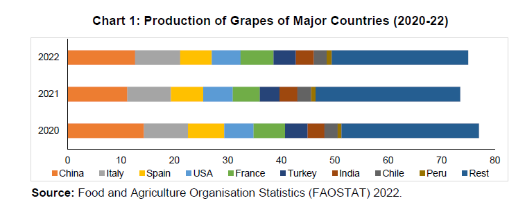
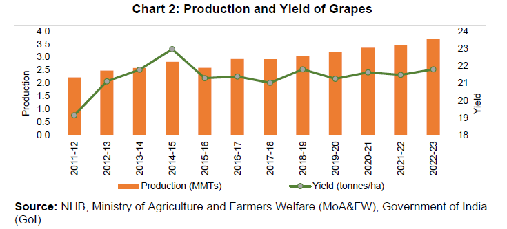
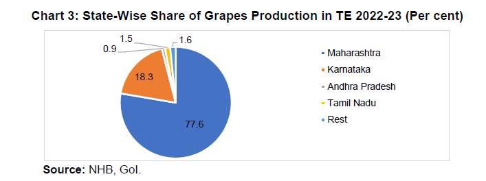
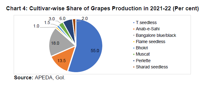
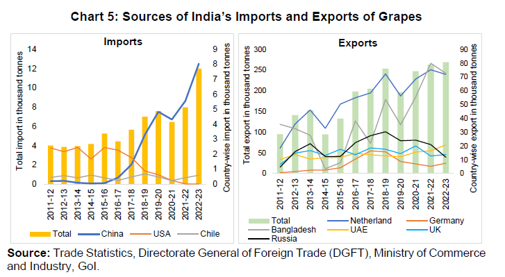
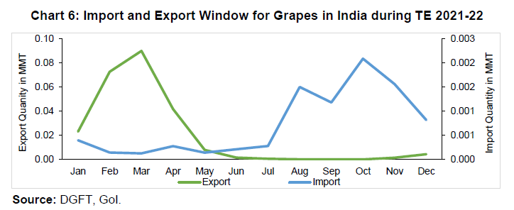
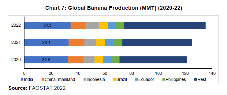
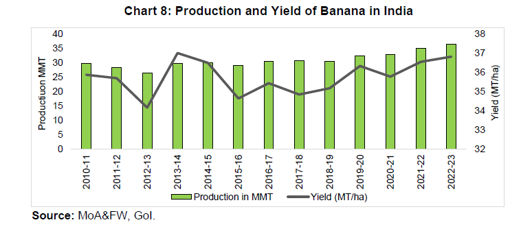
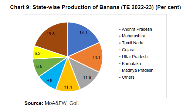
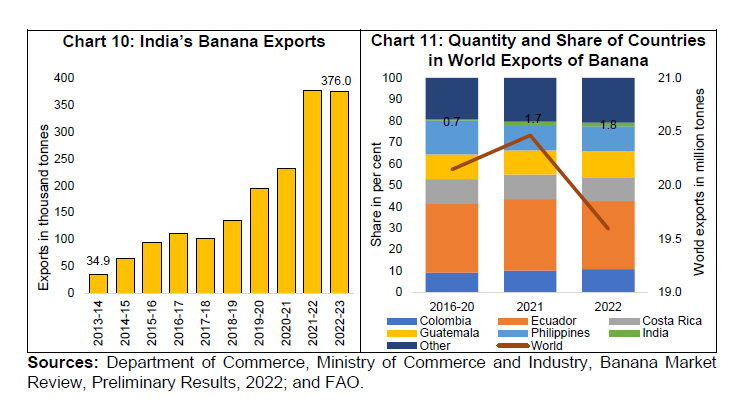
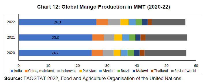
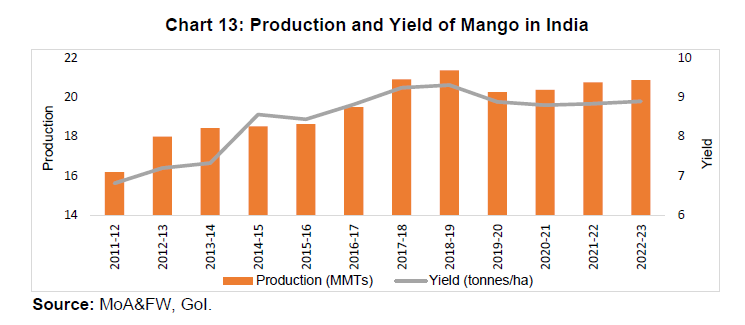
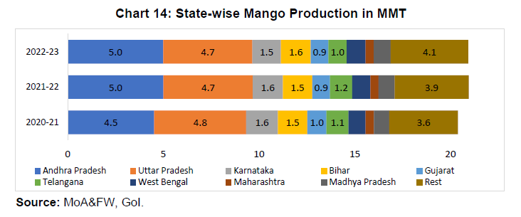
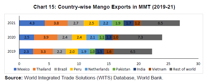
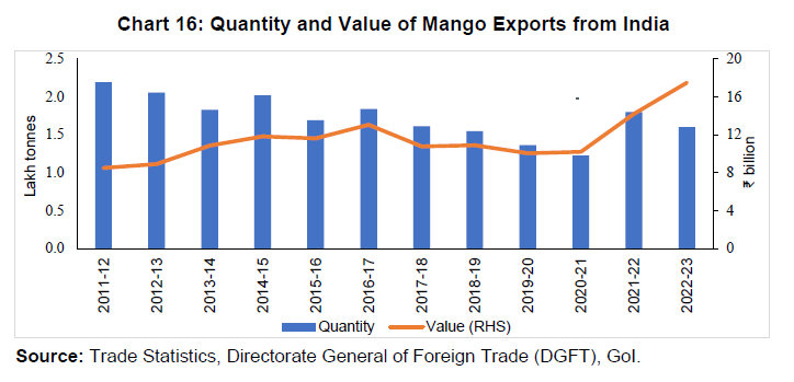
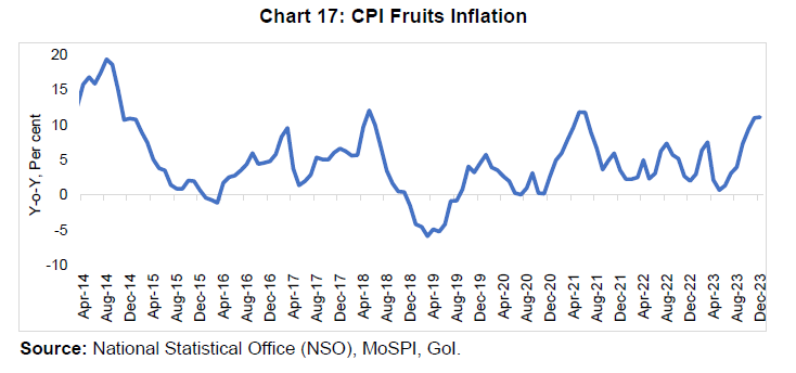
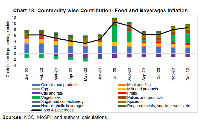
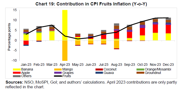
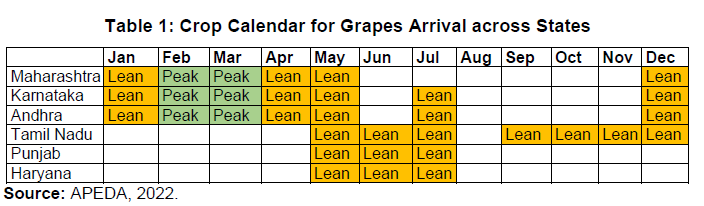
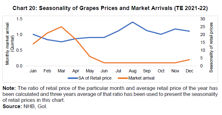
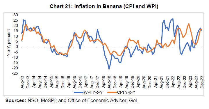
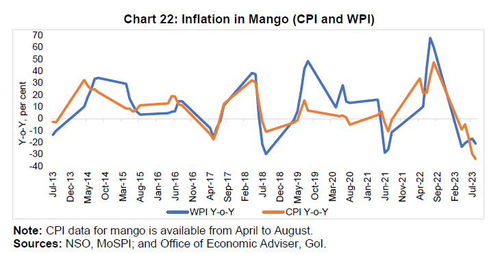
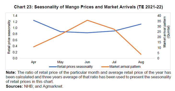
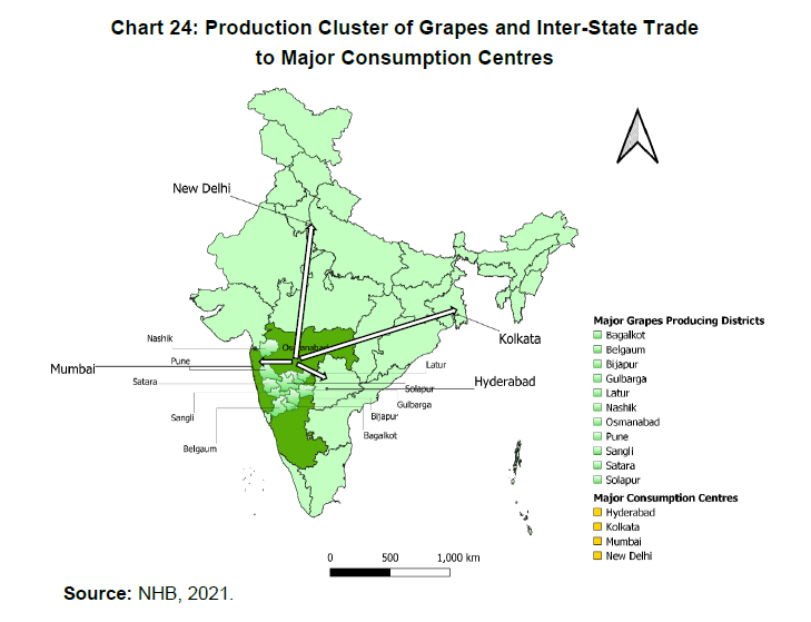
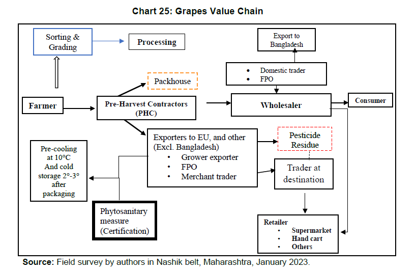
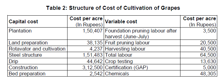
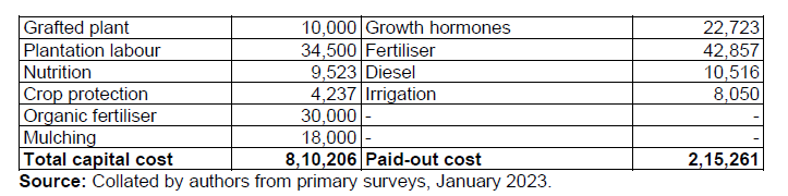
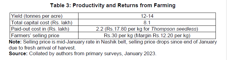
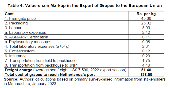
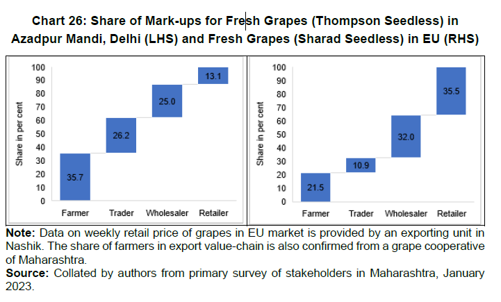
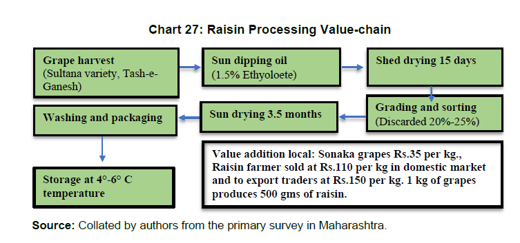
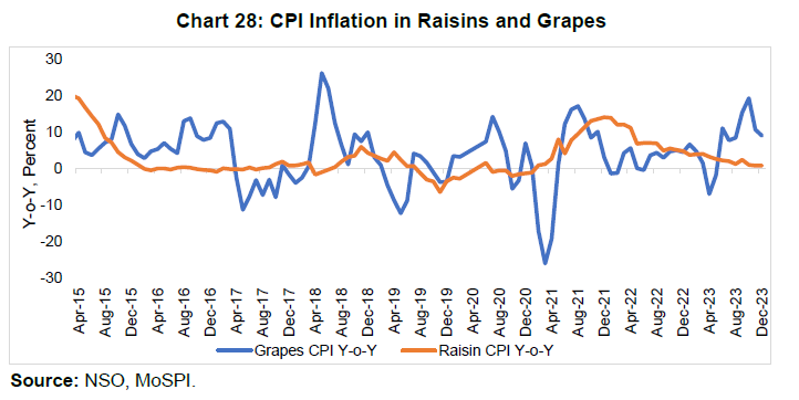
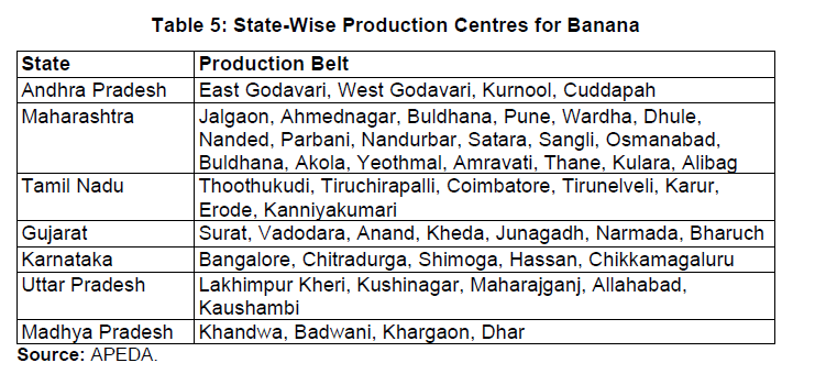
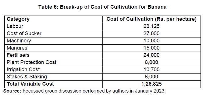
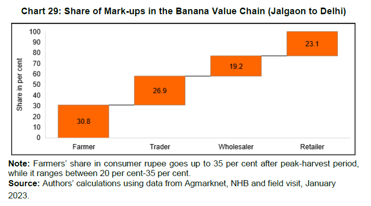
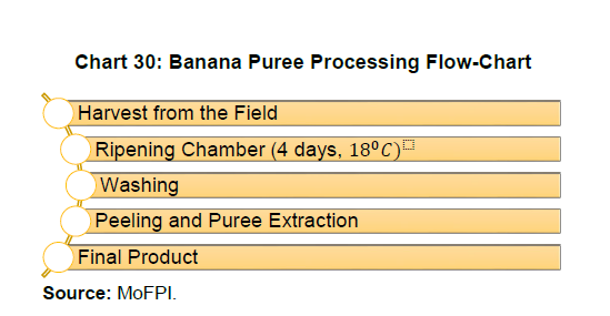
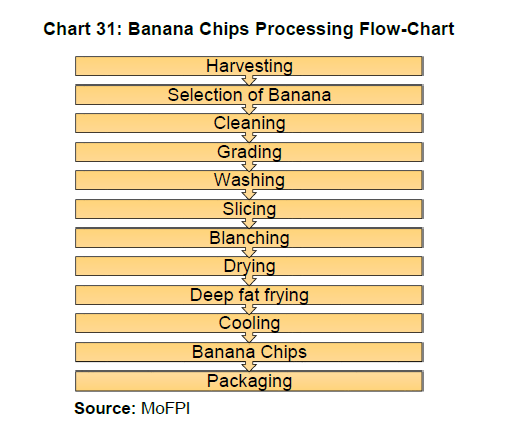
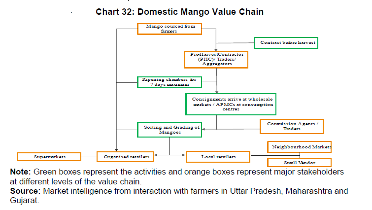
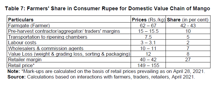
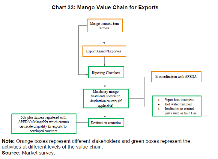
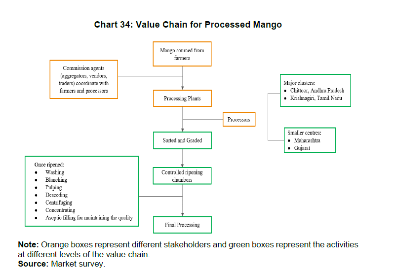
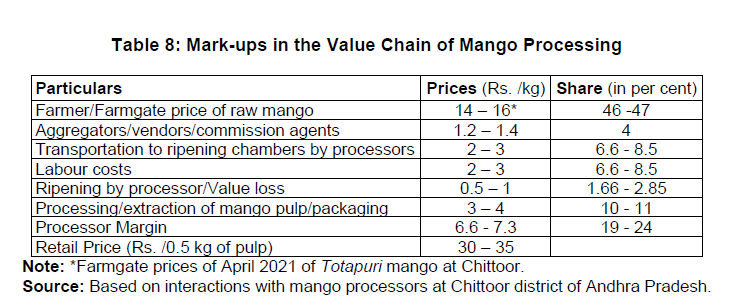


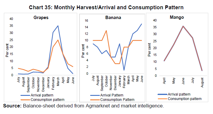


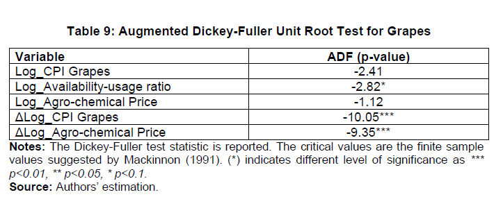
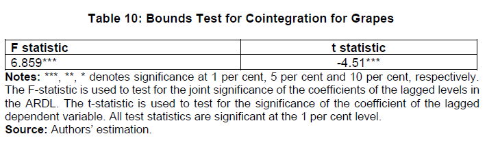
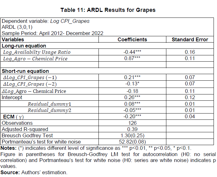
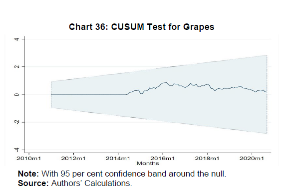
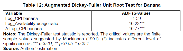
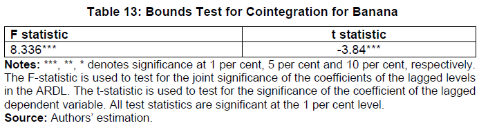
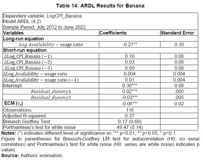
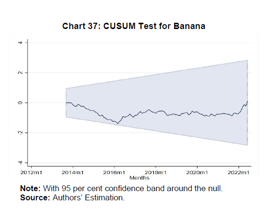
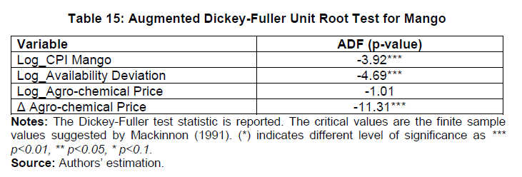
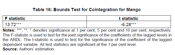
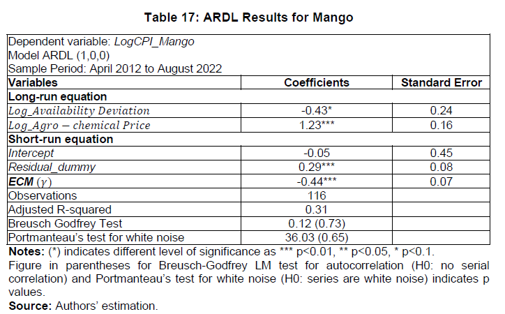
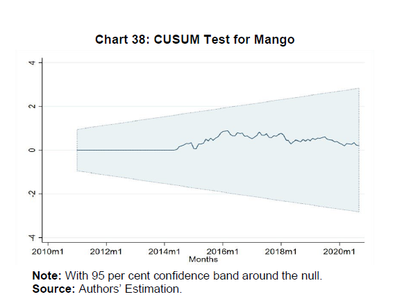
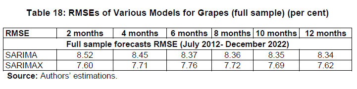
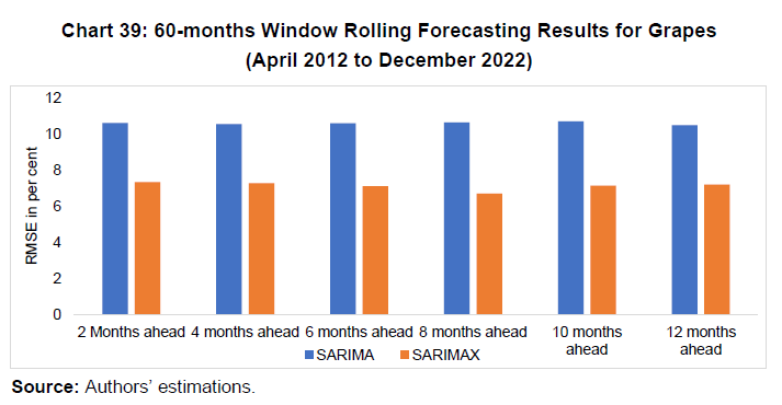
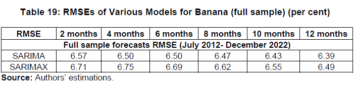
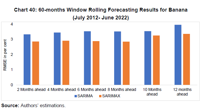
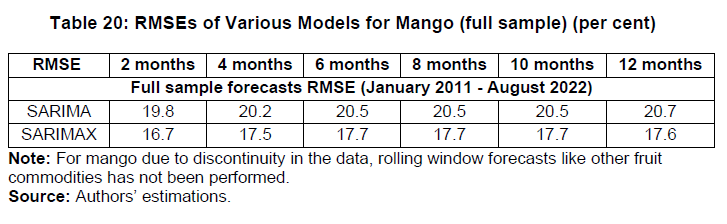
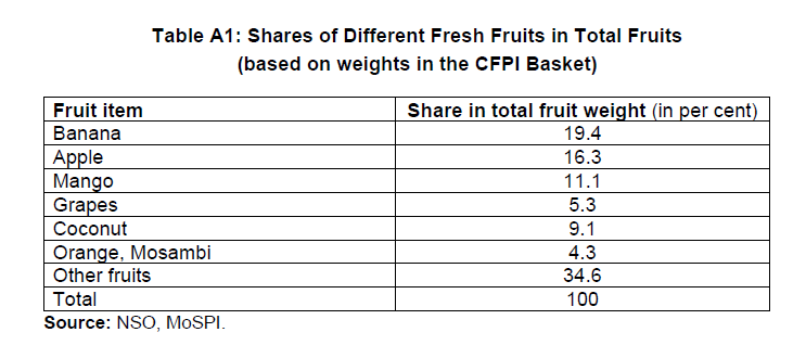
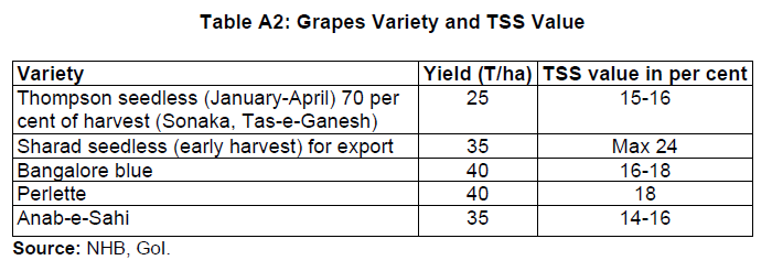
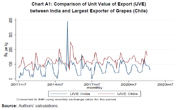
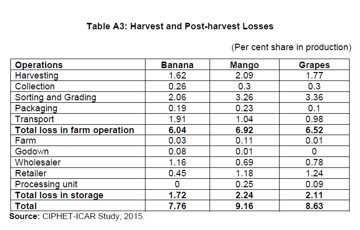
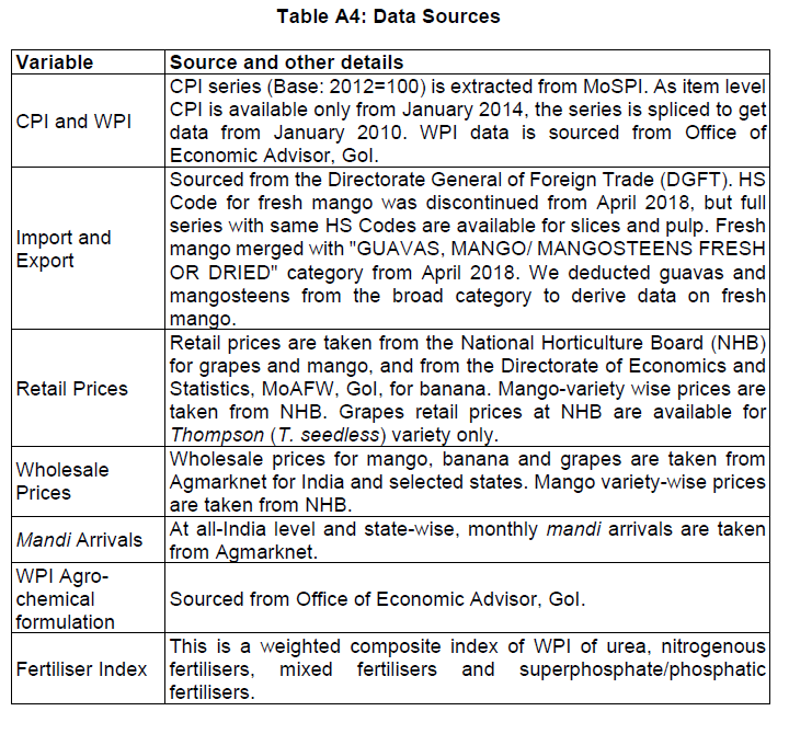
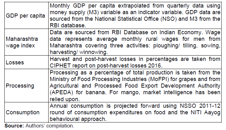

Share this page:


Install the RBI mobile application and get quick access to the latest news!
Scan the QR code to install our app


Page Last Updated on:


