Press Release

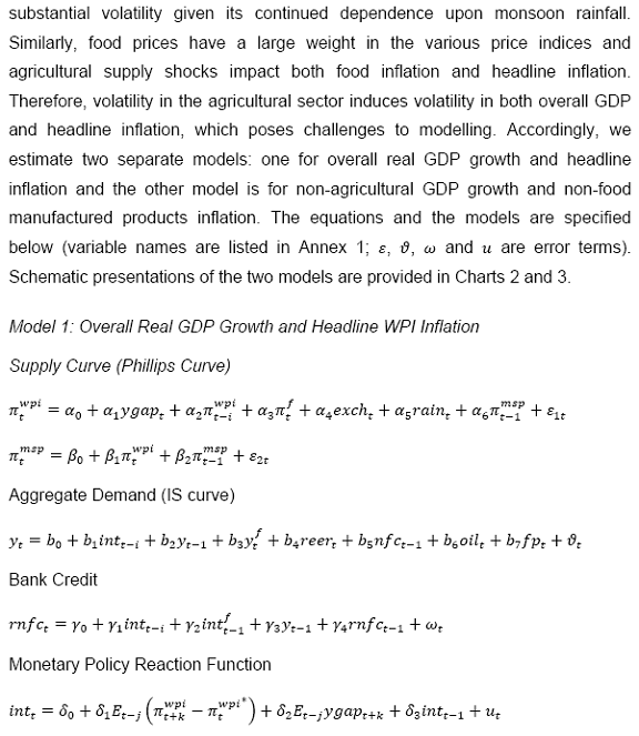
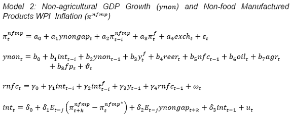
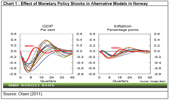
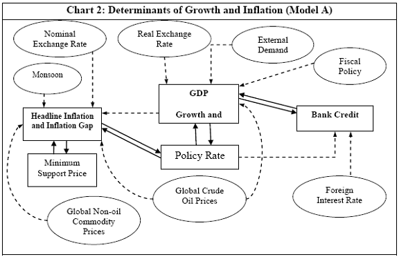
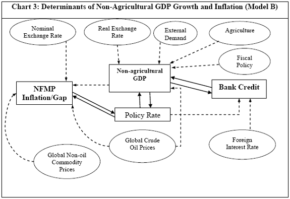
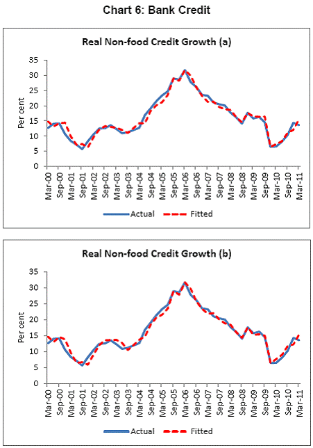
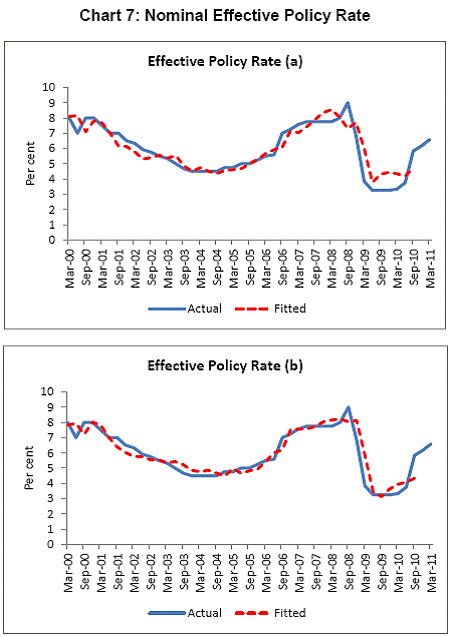
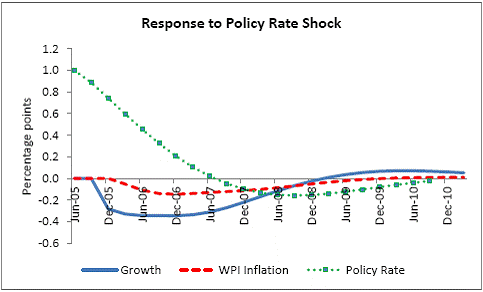
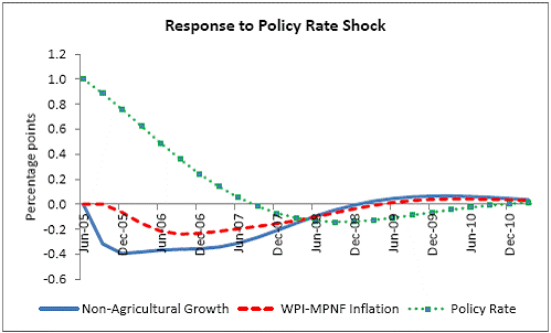
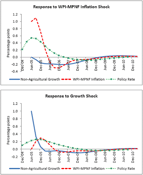
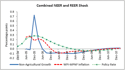
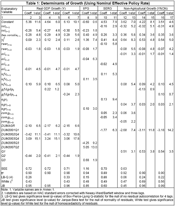
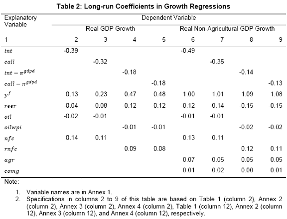
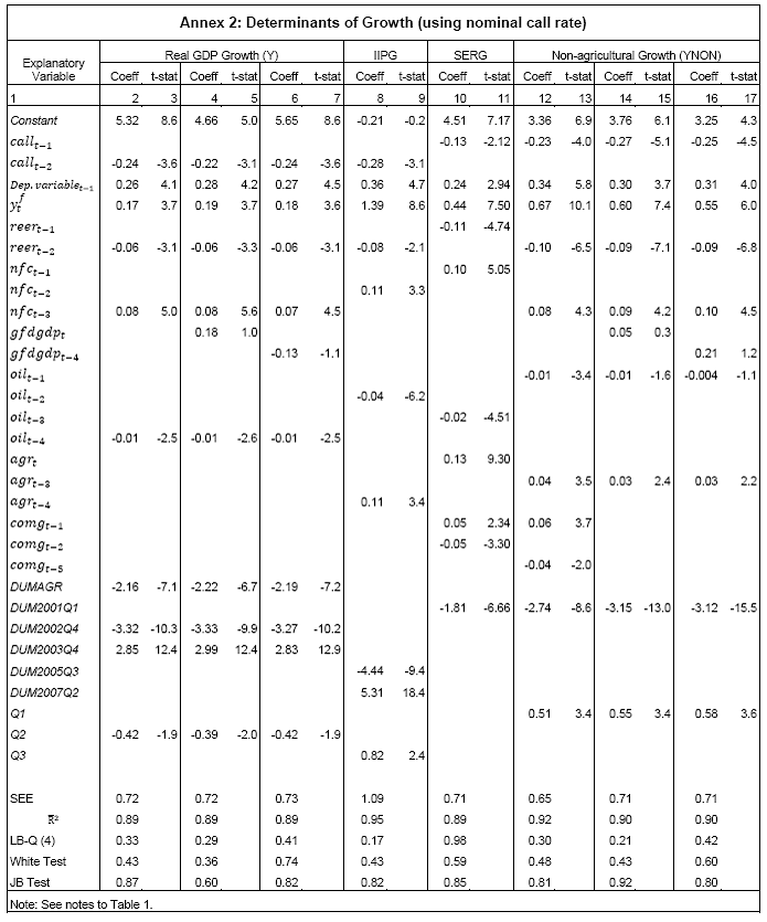
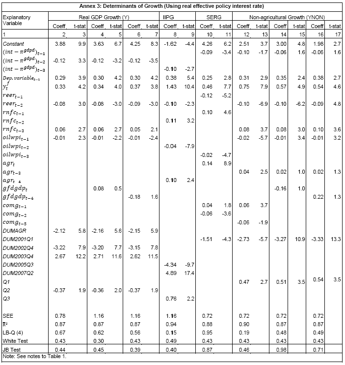
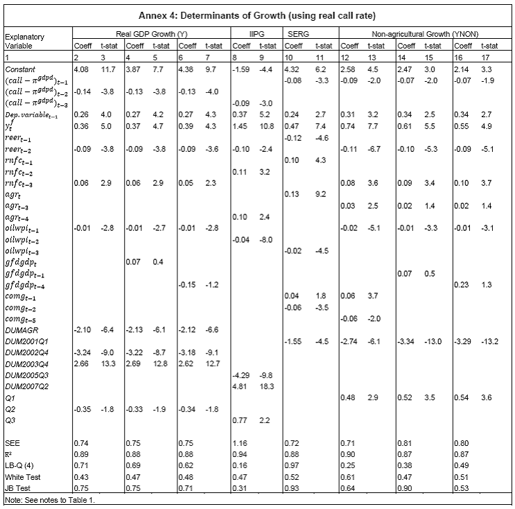
RBI Working Paper Series No. 09
Monetary Transmission Mechanism in India: A Quarterly Model
^@Muneesh Kapur and Harendra Behera

¹This paper examines monetary transmission mechanism for India in the context of a small macro model using quarterly data. Given the volatility emanating from the agricultural sector, the paper models both overall growth and overall inflation as well as non-agricultural growth and non-food manufactured products inflation, i.e., components stripped of the influence from the agricultural sector and which are more amenable to monetary actions. Model simulations for a one-quarter 100 bps increase in the nominal effective policy rate show that the peak effect on non-agricultural growth is almost 40 bps with a lag of 2 quarters and that on non-food manufactured products inflation is 25 bps with a lag of 5 quarters. Therefore, the interest rate channel is effective in the Indian context and the magnitude of the impact on growth and inflation is comparable to that in major advanced and emerging economies; however, the evidence for both India and other countries suggest that the impact of monetary policy actions on inflation is modest and subject to lags. The results are sensitive to alternative measures of real interest rate. Despite the monetary tightening by Reserve Bank of India during 2010 and 2011, inflation remained high and this could be attributed to the structural component of food inflation as well as the surge in international commodity prices beginning the second half of 2010 and continuing into the first half of 2011.

JEL Classification Numbers: E31; E32; E52; E58; F41

Keywords: Exchange Rate Pass-through, India, Monetary Policy, Monetary Policy Reaction Function, Monetary Transmission, Neutral Interest Rate, Phillips Curve.

Inflation in India was persistently high during 2010 and 2011. In response, monetary policy was progressively tightened beginning March 2010 – the effective policy rate was increased by 525 basis points (bps) from 3.25 per cent in March 2010 to 8.50 per cent in October 2011. Over this period, domestic growth slowed down, while inflation remained relatively sticky. The slowdown in growth was not only due to the monetary stance, but also the global economic recovery losing momentum over euro area sovereign debt concerns and domestic policy and regulatory concerns (RBI, 2011b).

According to the standard monetary transmission mechanism, variations in interest rates first impact aggregate demand and GDP growth, which, in turn, then impact inflation. Therefore, inflation management needs some temporary loss of output. To the extent that growth may be impacted, it must be understood as a short-term trade-off, with positive consequences for long-term performance (Gokarn, 2011). The Reserve Bank’s anti-inflationary stance has been criticised from two different directions – for being hawkish from one side and for being soft on inflation from the other side. The proponents of the first view argue that inflation is driven largely by supply shocks and monetary policy response to such inflation would only end up hurting growth. The criticism from the other side has been that the Reserve Bank was soft on inflation and this led to the persistence of inflation. Both these critiques cannot obviously be right at the same time (Subbarao, 2011).

In this context, as the Economic Survey 2011-12 (Government of India (GoI), 2012) observes, the question is: How sharp are the connections between monetary policy instruments and inflation? While the simple “correlation between the policy instruments and inflation is slender”, a “careful statistical analysis by putting in lags” indicates “that the policy instruments do have an impact on inflation with a lag.... Nevertheless, there is plenty of white noise and the correlations are far from perfect. So much so that there is room for a multiplicity of opinions about what constitutes optimal control... The RBI increasingly voiced concern that the fiscal deficit that the government was tolerating was too high and made its task of controlling inflation harder. There were some in government who felt that the monetary tightening, successively 13 times, was not having adequate impact on inflation and the hardening interest rates were instead impacting more on growth (pp. 25-26, GoI, 2012).

Against this backdrop, this paper assesses monetary transmission dynamics – the impact of monetary policy actions on demand, output and inflation - in India using a small model. The paper quantifies the impact of interest rates and other determinants on growth and inflation. It also models the response of the central bank to growth and inflation dynamics.

Section I briefly discusses the various transmission channels of monetary policy and assesses the cross-country empirical evidence. Section II sets out the model framework, while Section III presents the empirical findings. Section IV concludes.

I. Monetary Transmission Channels

There are four key channels of monetary transmission: (a) interest rate channel; (b) quantum channel relating to credit; (c) asset price channel; and (d) exchange rate channel (Boivin, Kiley and Mishkin, 2011; Bernanke and Gertler, 1995). The first channel - the interest rate channel - is the key channel of monetary transmission in market-based economies and refers to changes in domestic demand and inflation brought about by changes in the policy interest rate. Variation in the short-term nominal policy interest rate impacts the spectrum of long-terms interest rates and yields. Lower nominal rates, given sticky wages and prices, lead to lower real rates. The resultant reduction in cost of credit encourages investment and consumption demand, which eventually gets reflected in an increase in output and prices.

The quantum channel - the credit channel - complements and amplifies the interest rate channel. The credit channel operates through the availability of bank credit (the traditional bank-lending channel or the narrow credit channel) and through the impact of interest rates on asset prices, and cash flows and net worth of borrower’s (the broader credit channel, or the balance-sheet channel or the net worth channel). For bank-dominated economies, the narrow credit channel is important and for financial market-dominated economies, the broader credit channel is important.

The asset price channel – the impact of changes in interest rates on movements in asset prices like real estate and equity prices - generate wealth effects in terms of market valuations of financial assets and liabilities, which then impacts consumption and investment. Finally, the exchange rate channel - higher domestic interest rates induce an appreciation of the domestic currency – has a direct impact on domestic prices (appreciation of the domestic currency makes imported goods cheaper) and aggregate demand (appreciation reduces net exports and hence demand).

The various channels are not mutually exclusive and there is considerable feedback and interaction among them. The relative importance of each channel may differ from one economy to another as well as over time for any given economy depending on a number of factors such as the degree of monetisation of the economy, the extent to which households borrow from the formal financial system, the state of development of financial markets, the instruments available to monetary policy, the fiscal stance and the degree of openness.

Empirical Evidence: Cross-Country

Cross-country studies of monetary transmission show lagged impact of monetary impulses on growth and inflation. For instance, in a vector autoregression (VAR) framework, for the US economy, output, consumption, investment and inflation display a hump-shaped response; the peak effect on output is found to occur about 1.5 years after a monetary policy shock and on inflation after about 2 years (Christiano et al., 1999). Boivin et al. (2011) compare the impact of monetary policy shocks for the period 1962Q1–1979Q3 with the period 1984Q1–2008Q4 in a factor-augmented VAR (FAVAR) model as well as a dynamic stochastic general equilibrium (DSGE) model for the US. According to the FAVAR model, the magnitude of responses of real GDP was greater in the pre-1979Q3 period than in the post-1984Q1 period, but the response in the later period was more delayed and persistent; the response of prices was considerably reduced in the post-1984Q1 period, compared to the earlier period, which these authors attribute to better anchoring of inflationary expectations. The results are qualitatively similar in their DSGE model, but there are important differences from the FAVAR responses - inflation and output jump following a policy innovation in the DSGE model, whereas the identifying assumption underlying the FAVAR responses excluded this possibility. According to the DSGE model results, during the 1984Q1-2008Q4 period, an increase of 100 bps in the policy rate reduces real GDP by around 40 bps with a lag of 2 quarters and inflation by around 30 bps with a lag of 3 quarters².

Els et al. (2003) examine monetary transmission in the euro area across a range of models – a VAR model and three macro models. For an increase of 100 bps in the interest rate (maintained for two years), they find that the maximum effect on output is reached in the first 1-2 years and GDP contracts by 20-40 bps after 1 year and by 30-70 bps after 2 years across models. The effect on prices is felt more slowly and is more persistent. Prices decline by 20-40 bps after 3 years.

For the United Kingdom, according to the Bank of England’s (BoE’s) macro model, in response to an increase of 100 bps in interest rates (increased for 4 quarters), the peak decline in output is 0.3 per cent (after about a year) and output returns to the baseline after 3 years. Inflation is broadly unchanged during the first year and the peak decline of 0.3 per cent occurs by the beginning of the third year (Bank of England, 2000). These results broadly carry through the BoE’s DSGE model (the Bank of England Quarterly Model, BEQM). The notable differences vis-à-vis the earlier macro model are: first, the demand effects come through a little more quickly in the BEQM, reflecting the stronger short-run response of consumption to interest rate changes in the BEQM; second, the effects of the temporary change in interest rates on inflation are somewhat less persistent in the BEQM, reflecting forward-looking households and firms who expect monetary policy will be set so as to return inflation to the base (Bank of England, 2004).

Similar growth-inflation dynamics and lags are corroborated by more recent studies for other countries. For Sweden, a one-quarter 100 bps increase in the policy rate reduces output by 50 bps (peak effect) and inflation by 20 bps (peak effect) after 6 quarters according to MOSES³, the aggregated econometric model for Sweden (Bardsen et al., 2011). For Norway, the peak decline in output is 40-70 bps (lag of 5-6 quarters) across a range of VAR models while that in inflation is 20-30 bps (lag of 9-11 quarters) following a one-period tightening of 100 bps; according to the Norges Bank’s macro-model (NEMO), the peak decline in output and inflation for a similar monetary policy shock is 40 bps (after 4 quarters) and 25 bps (after 2 years) (Olsen, 2011). In response to a similar monetary policy shock, for Japan, the peak decline in output and inflation is 14 bps (after 7 quarters) and 4 bps (after 10 quarters) according to the Bank of Japan’s large-scale hybrid-type macro model (Fukunaga et al., 2011). The relatively smaller impact of monetary policy on output and prices in Japan could perhaps be a reflection of the reduced efficacy of monetary policy in view of near zero policy interest rates since the mid-1990s.

The transmission lags in emerging market economies broadly follow a similar pattern as in key advanced economies, albeit the lags are shorter in some cases. The interest rate channel gained importance in the EMEs during the 2000s (Mohanty and Turner, 2008). During the 2000s, monetary policy frameworks in the EMEs became more credible, and central banks were more flexible in their operations, benefitting from reduced fiscal dominance and greater exchange rate flexibility. These shifts and the associated balance sheet changes strengthened the interest rate channel and inflation in most EMEs became lower and less volatile. Mukherjee and Bhattacharya (2011) assess monetary transmission mechanism in select inflation targeting EMEs in a panel regression framework and find that private consumption and private investment decline by 26 bps and 46 bps in response to an increase of 100 bps in real deposit rate and real lending rate, respectively.

Turning to select country experiences, for Poland, a hike in short-term interest rates of 100 bps sustained for 4 quarters results in a reduction in GDP growth of 30 bps after 4 quarters and a reduction in inflation of 20 bps after 8 quarters (Pruski and Szpunar, 2008). In Brazil, a one-period 100 bps increase in interest rate leads to a peak decline of 12 bps in output after 2 quarters (cumulative decline of 23 bps in output in the first year), while inflation decline peaks at just under 40 bps in the third quarter. The bulk of the effects on both output and inflation take place within 4 quarters. The transmission lags are thus shorter than in advanced economies, attributable to factors such as shorter maturity of domestic credit, and the considerable weight of the exchange rate in domestic currency pricing (Catão et al., 2008). For Chile, the results from a structural model indicate that a one-quarter 100 bps increase in the interest rate reduces output by 60 bps (the peak effect) after 1 quarter; the peak reduction in inflation is 25 bps after 7 quarters (Garcia et al., 2005).

In Mexico, exchange rate fluctuations have become less important in the determination of prices, while interest rate movements have had a faster and stronger effect on inflation on the back of the expectations channel of monetary policy (Sidaoui and Ramos-Francia, 2008). For some EMEs, the exchange rate channel remains a dominant force. For example, for Indonesia, in the post-Asian crisis period, exchange rate movements have become more pronounced in affecting output and prices, while the effectiveness of monetary policy to influence the exchange rate has been undermined with exchange rate movements being driven more by non-economic factors. Although the interest rate channel still works quite well in transmitting monetary policy, its magnitude has been affected by conditions in the banking system and overall higher uncertainty and risk factors (Goeltom, 2008). For Hungary, prices are affected in the first year after an increase in the policy rate and the response is persistent. However, output reacts only marginally as the drop in investment after monetary tightening is offset by pick-up in consumption; the output response is mitigated by short-run nominal wage rigidity and the quick exchange rate pass-through, as a result of which the income effect offsets the interest rate effect on consumption (Vonnák, 2008).

To summarise, the cross-country empirical evidence indicates that the peak effect of monetary policy on output and inflation in advanced economies occurs after a lag of around 4 and 6 quarters, respectively. The lags appear to be relatively shorter in EMEs. The peak effect of an increase of 100 bps in interest rate is around 30-70 bps on output and around 20-40 bps on inflation. However, the transmission lags as well as the impact of monetary policy on growth and inflation can change over period as well as across models as documented, for example, by Olsen (2011) for Norway (Chart 1).

Empirical Evidence: India

Monetary transmission dynamics for the Indian economy have been studied in a number of studies using alternative approaches. VAR approaches have been used to assess various aspects of transmission, inter alia, in Ray, Joshi and Saggar (1998), Al-Mashat (2003), RBI (2004), Aleem (2010), Bhattacharya et al. (2011), and Khundrakpam and Das (2011). New Keynesian model (NKM) to assess transmission has been estimated in RBI (2002), and Patra and Kapur (2012) and calibrated in Goyal (2008) and Anand et al. (2010). Individual equations of the NKM have also been estimated in a number of papers, with most of them concentrated on the Philips curve [for example, Kapur and Patra (2000), Dua and Gaur (2009), Paul (2009), Patra and Ray (2010), Mazumdar (2011), Singh et al. (2011)]. Taylor-type rules have been examined in Mohanty and Klau (2004), Virmani (2004), Srinivasan et al. (2008), Takeshi and Hamori (2009), Anand et al. (2010), Hutchison et al (2010), and Singh (2010)⁴.

RBI (2004) analysed monetary transmission through a VAR using the index of industrial production, wholesale price index, Bank Rate, broad money and exchange rate. The peak effect of an interest rate shock on output and inflation occurred after 6 months, consistent with evidence of shorter lags in EMEs. The lags are corroborated by Aleem (2010) who find that the peak decline in both GDP and prices occurs in the third quarter after the interest rate shock. Mohanty (2012), using a quarterly structural VAR (SVAR) model, finds that policy rate increases have a negative effect on output and inflation; the peak effect on output growth takes with a lag of two quarters and that on inflation with a lag of three quarters. The overall impact persists through 8-10 quarters. These results are found to be robust across alternative specifications with different measures of output, inflation and liquidity. Anand et al. (2010) employ a DSGE model framework and their results indicate that the peak effect of a 100 bps increase in the nominal policy rate (call rate) is 35-45 bps on output and around 15 bps on inflation and the peak effect on both output and inflation is felt in the first quarter after the policy rate shock.

In contrast, according to Bhattacharya et al. (2011), the interest rate channel in India is weak and the most effective mechanism is the exchange rate channel. According to their long-run cointegrating relationship, an increase of 100 bps in the call money rate has a negligible impact on industrial production (their activity variable) and a reduction of only 1 bps in inflation; in comparison, one per cent currency depreciation increases inflation by 20 bps. The impact of interest rate on inflation is not direct, but through the exchange rate channel: higher interest rates lead to appreciation of domestic currency, which then impacts inflation. Similarly, Bhalla (2011) is sceptic about monetary policy’s ability to contain inflation; according to him, “there is no evidence - zero -  to link the decline in India’s inflation rate post 1996 to Indian monetary policy, while there is a lot to link the decline in India’s GDP growth rate to this very same policy”. Goyal (2008) finds that a monetary stimulus preceding a temporary supply shock can abort inflation at minimum output cost, on account of exchange rate appreciation, accompanying a fall in interest rates and rise in output.

Given the bank-dominated financial system, the credit channel has also been focus of studies. RBI (2010) reports evidence in favour of credit channel in the context of VAR model. Increase in call money rate leads to lower growth in non-food credit in the fifth quarter and GDP growth in the seventh quarter. The estimated impact is found to be modest and tapers off gradually. The causality running from GDP growth to credit growth turns out to be statistically significant, suggesting credit following, rather than leading the pick-up in growth momentum. Khundrakpam (2011) finds the credit channel to be significant and robust. An increase of 100 bps in the policy rate was found to reduce bank credit by 2.2-2.8 per cent. Pandit and Vashisht (2011) examine the credit channel for India and six other EMEs in a panel regression framework and find that the policy rate is an important determinant of firms’ demand for bank credit, which confirms the role of countercyclical monetary policy tool for setting the pace of economic activity. Banerjee (2011) examines the direction of credit-output causality for the period 1950-2011 and finds changes in the causality direction over the period: output was predominantly driven by credit in the pre-1980s period, nearly no relationship between the two during the 1980s and credit being primarily driven by output in the post-reforms period. For the non-agricultural sector as a whole, the unidirectional causality from output to credit in the post-reforms period stressed the importance of output in determining the quantum of flow of credit. However, at the industry level, a few industries exhibited bidirectional causality.

Khundrakpam and Das (2011) examine the relative response of food and manufactured products prices to change in interest rate and money supply. They find that, in the long-run, variations in money supply impact prices of both food and manufactured products prices but the impact of money supply is more on food prices than on manufactured products prices; in contrast, variations in call rate have a negative effect only on manufactured products prices. Their findings suggest that the quantum channel is more potent vis-a-vis the interest rate to deal with supply shocks.

II. The Model

The key approaches to study monetary transmission are estimation of VAR models or macro models. While the VAR-based approach is quite popular in empirical research, its key limitation is the atheoretic nature and the number of variables it can handle in the context of short-sample periods. This limitation is especially relevant in the Indian context since quarterly GDP data are available from 1996 onwards. Moreover, VAR studies have typically focussed on the transmission lags, while being silent on the impact of monetary policy on growth and inflation, which are critical input for monetary policy calibration. A number of studies in the Indian context have used monthly IIP data as an indicator of economic activity. Inflation reflects overall demand-supply mismatches in the economy. Industrial sector accounts for less than a fifth of total GDP in India and hence it could be a misleading indicator of demand pressures in the economy. Finally, the VAR approach implicitly assumes a backward-looking monetary policy reaction function. In the actual world, given the monetary lags, monetary policy has to be forward-looking and needs to responds to expected inflation and growth and not their past values. For India, the evidence in Patra and Kapur (2012) shows that a forward-looking monetary policy reaction function yields coefficients consistent with the Taylor principle (and hence are stabilising), while the backward-looking reaction function results in the inflation coefficient below unity. Thus, a VAR-based approach could end up with misleading conclusions. Residuals from the VAR regressions used to represent exogenous policy shocks often bear little resemblance to standard interpretations of the historical record of policy actions and the VAR residuals differ across specifications (Walsh, 2010).

Notwithstanding these limitations, the VAR framework remains an important approach to assess monetary transmission and provides a useful method to corroborate findings from alternative methodologies. In the Indian context, given the still limited studies on monetary transmission, it would be useful to explore alternative approaches to study the transmission mechanism, including the VAR framework. It would also be interesting to assess the forecasting performance of alternative approaches. For example, Hammersland and Traee (2012) compare forecasting performance for a structural model with AR and VAR models for Norway and find: first, the accuracy of the structural model is better than AR and VAR for forecasting wage inflation and GDP growth on all horizons; second, the VAR model is the best on all horizons for forecasting core inflation, the rate of unemployment, the lending rate and the real exchange rate; and, finally, the relative advantage of the structural model seems to increase with the forecast horizon. Thus, alternative modelling approaches may be needed to have robust forecast for variables of interest to monetary policy.

In view of the above debate and in order to explore and develop alternative approaches, this paper prefers to examine monetary transmission dynamics in India through the estimation of a small model, drawing from the New Keynesian perspectives (Clarida et al. 1999; Woodford, 2003; Gali, 2008) and empirical studies on the various building blocks of the NKM (Gali and Gertler, 1999; Goodhart and Hoffman, 2005 a, b; Taylor, 1993; Clarida et al. 1998, 2000; Paez-Farrell, 2009).

While the New Keynesian model is purely forward-looking, available empirical evidence is mixed. In particular, the New Keynesian Philips Curve (NKPC) and its forward-looking character is debatable. While Gali and Gertler (1999) and Gali, Gertler, and Lopez-Salido (2005) argue in favour of NKPC, Rudd and Whelan (2007) argue that its empirical estimates are subject to serious identification issues. The NKPC specification does not distinguish forward-looking models from backward-looking models; the higher weight on expected inflation found by the proponents of NKPC may be due to misspecification resulting from omission of explanatory variables from the main equation. Typically, expected inflation is instrumented through lagged inflation amongst the instrument set and this can bias the coefficient of expected inflation to be higher and NKPC can yield large estimates of the coefficient of expected inflation even when forward-looking behaviour is completely absent.

In view of the above debate, this paper builds upon the evidence presented in Patra and Kapur (2012), who estimate a range of specifications - purely forward looking, backward-looking and hybrid versions - for the three key equations of the NKM, viz. the IS curve, the Philips curve and the monetary policy reaction function; their results favoured a forward-looking monetary policy rule, but backward-looking Phillips curve and IS curve. In view of these findings, we estimate a forward-looking monetary policy rule (following Clarida et al. 1998, 2000; Paez-Farrell, 2009) and backward-looking Phillips curve (following Gordon 1998, 2011) and IS curve (following Goodhart and Hoffman, 2005 a, b).

This paper extends the analysis in Patra and Kapur (2012) in a number of directions. First, apart from overall GDP, this paper also focuses on its major components (industry, services and non-agricultural GDP). Second, given the monetary policy interest in the impact of policy actions on real GDP growth, the IS curve analysis in this paper is in terms of growth rates of output than that in terms of output gaps. Third, alternative indicators of real interest rates are used in this paper to assess the sensitivity of results. Fourth, given the focus of monetary policy on non-food manufactured products inflation as an indicator of demand-side pressures, non-food manufactured products inflation dynamics have also been modelled in addition to headline inflation. Fifth, and related to the previous point, two variants of monetary policy reaction functions are modelled:  one as responding to headline inflation and overall GDP and the other responding to non-food manufactured products inflation and non-agricultural GDP. Sixth, the analysis also attempts at assessing the impact of oil prices, bank credit and fiscal policy on output. Seventh, the influence of minimum support prices and monsoon rainfall on inflation and the feedback from headline inflation to minimum support prices are also analysed. Eighth, determinants of non-food bank credit are also assessed. Finally, this paper extends the analysis to the quarter ended March 2011.

We, therefore, estimate the following model. First, following the Phillips curve approach, inflation is modelled as a function of domestic demand conditions, supply shocks, rainfall conditions, trends in minimum support prices and inflation expectations (proxied by lagged inflation). Second, minimum support prices are endogenised, given their role in the inflation process. Third, following the IS curve framework, output growth is assumed to depend upon interest rate, bank credit, asset prices, external demand, oil prices and real exchange rate. As discussed later, we estimate growth equations separately for nominal and real interest rates to check sensitivity to the choice of the interest rate as also to have some comparability with the VAR literature. Fourth, in view of the dominance of the banks in the credit system, determinants of demand for bank credit are modelled. Finally, the monetary policy reaction function is estimated on the lines of a Taylor rule, with the policy rate reacting to deviations of inflation from the inflation target/objective and the output gap.

Although the share of the agricultural sector in GDP has declined over the years, it remains significant. At the same time, the agricultural output exhibits

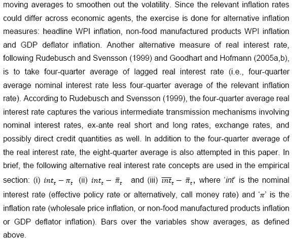
Real Interest Rate

While the model specifications above show nominal interest rates in the aggregate demand equations, sensitivity of results to the use of nominal as well as real interest rates is attempted in the empirical exercise. In theory, real interest rates matter for consumption and investment decisions; however, most of the media commentary as well as discussions by corporates is typically in terms of nominal interest rates rather than real rates. According to Fair (2012), households appear to respond more to nominal rates than to real rates. Moreover, the appropriate measure of real interest rate remains contentious. In principle, real interest rate is nominal interest rate less expected inflation. How does one measure expected inflation? The relevant measure of inflation for the purpose of computing real interest rate remains a matter of debate (Gokarn, 2011). The relevant inflation rate could also differ for different economic agents in the country (Mohan, 2002).

In the absence of a consistent series on inflation expectations, this paper attempts alternative measures of real interest rate. Assuming adaptive expectations, expected inflation is proxied by following alternative measures: current year-on-year (y-o-y) inflation on the one hand and its 4- and 8-quarter

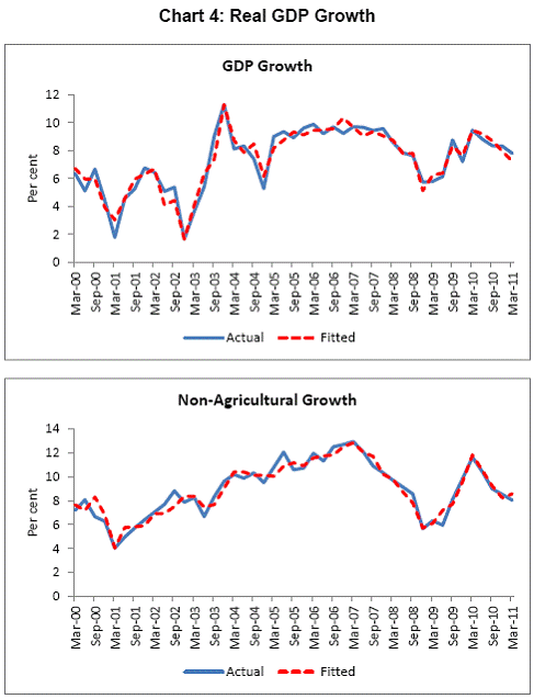
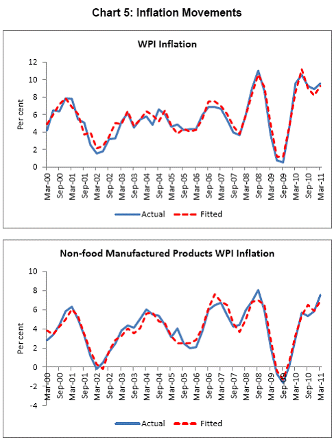
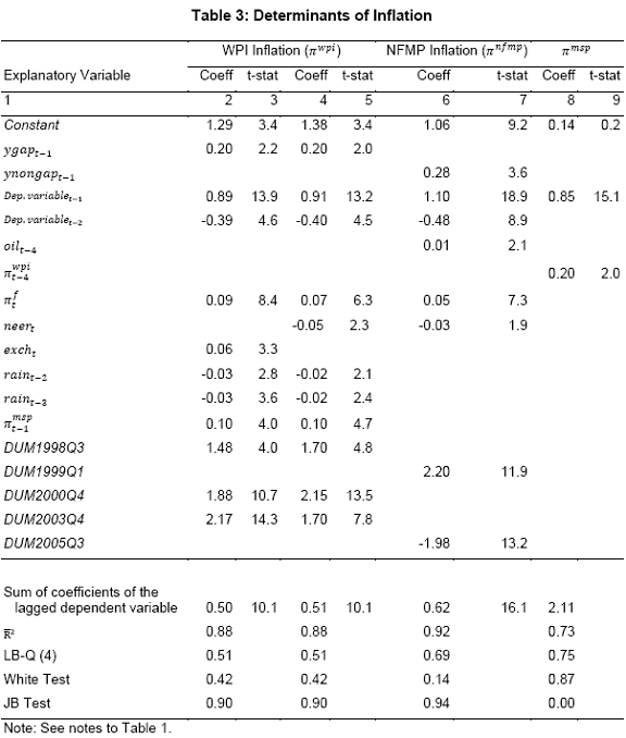
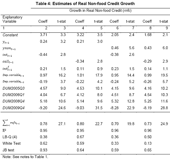
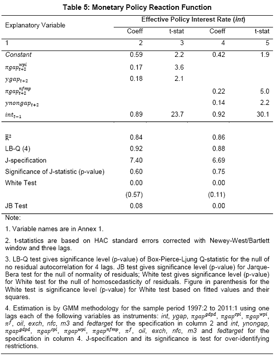
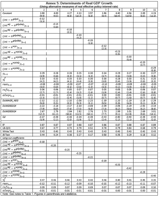
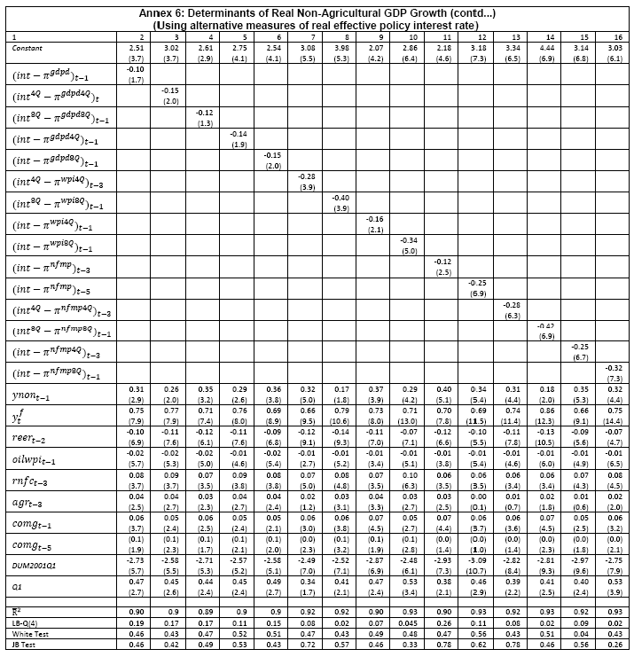
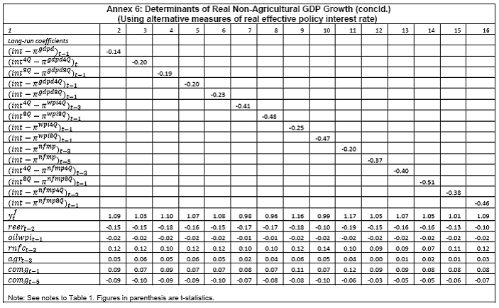
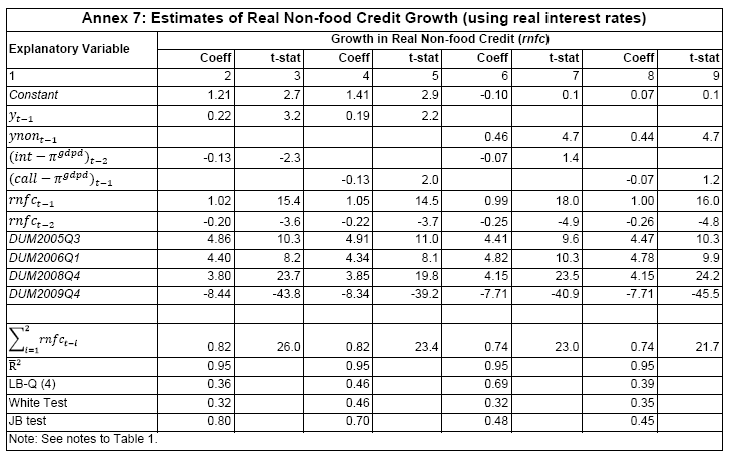
III. Data and Estimation Results

Data

The paper uses quarterly data from the quarter April-June 1996 onwards – the period from which quarterly GDP data are available – up to the quarter ended March 2011. While year-on-year growth rates of various variables are based on actual data series, output gap measures are based on seasonally adjusted data. All the data series are stationary⁵.

As regards the appropriate policy interest rate, the choice is complicated by substantial changes in the monetary policy framework and operating procedures over the period of the study. The Reserve Bank switched from the monetary targeting framework to a multiple indicators framework in 1998. The Bank Rate was re-activated in 1997. In the early 2000s, the liquidity adjustment facility (LAF) was introduced to manage liquidity through repo (liquidity injection) and reverse repo (liquidity absorption) operations. From 2003 till May 2, 2011, monetary policy signals were provided through changes in both repo and reverse repo rates in conjunction with variations in the cash reserve ratio (Mohan, 2009; Mohan and Kapur, 2009). During episodes of excess liquidity (2001 through 2006 and again from 2008:4 to 2010:2), the reverse repo rate was the effective policy rate. On the other hand, during episodes of monetary tightening/liquidity shortage (2007:1 to 2008:3 and 2010:3 to 2011:4), the repo rate became the effective policy rate. Thus, the policy rate, during the post-2003 period, switched between repo and reverse repo rates. Overall, the Bank Rate was the effective policy rate for the first few years of the sample and in the subsequent period, repo/reverse repo rate was the effective rate. The effective policy rate, thus defined, is used as the policy rate as in Patra and Kapur (2012).

An alternative to the effective policy rate series would be to use call rate data, as a number of studies have done; however, the call rates move in response to the short-term liquidity conditions and, at times, have overshot the operative policy rate, which can impart avoidable noise to the series. Nonetheless, as a measure of robustness check, the paper also estimates and reports the impact when call rate is used as the policy rate.

As noted earlier, the operating policy rate alternated between repo and reverse repo rates from 2003 till the end of the sample period (2011:1), depending upon the prevailing liquidity condition. Thus, there was the lack of a single policy rate. Against this background, the operating framework was modified effective May 3, 2011. First, the repo rate was made the only one independently varying policy rate to transmit policy signals more transparently. Second, a new Marginal Standing Facility (MSF) was instituted under which scheduled commercial banks (SCBs) can borrow overnight at their discretion up to one per cent of their respective NDTL at 100 bps above the repo rate to provide a safety valve against unanticipated liquidity shocks. Third, the revised corridor was defined with a fixed width of 200 basis points. The repo rate was placed in the middle of the corridor, with the reverse repo rate 100 bps below it and the MSF rate 100 bps above it (Mohanty, 2011).

Estimation Results⁶

Growth Dynamics

We model overall real GDP growth as well as its two major components, viz, industry and services separately and collectively as non-agricultural growth. The services sub-sector ‘community, social and personal services’ is impacted by fiscal policy actions directly and given its high volatility, the estimates for services and non-agricultural growth exclude this component of services⁷. As noted earlier, we test for the sensitivity of the results to the use of both nominal and real interest rates. In the specifications with the nominal interest rate, non-food credit and oil inflation are also used in nominal terms; in the specifications with the real interest rate, non-food credit and oil inflation are used in real terms.

Beginning with the specifications using the nominal policy rate, key findings are: first, the policy interest rate has a statistically significant negative impact on overall growth as well as its major components with a lag of 1 to 2 quarters. An increase of 100 bps in the policy interest rate reduces overall GDP growth by 28 bps with a lag of two quarters and the long-run impact is 39 bps (Table 1, columns 2 and 12). The long-run impact of a similar increase in the policy rate on non-agricultural growth is 50 bps (Table 2). Second, non-food credit has a positive and significant impact on economic activity, controlling for the impact operating through the interest rate variable. This suggests that both the interest and the credit channel of monetary policy transmission are important.

Third, global economic conditions have a positive and statistical significant impact on domestic activity. An increase of one percentage point in global GDP increases non-agricultural GDP by a similar order in the long-run; the impact is found to be quite sizable (225 bps) in the case of industrial production. Fourth, the real exchange rate appreciation has the expected dampening impact on economic activity, with a lag of 1-2 quarters: 10 per cent real appreciation reduces real GDP growth by 40 bps and non-agricultural GDP growth by 120 bps in the long-run.

Fifth, oil prices are found to have a negative impact on output with a lag of 1 to 4 quarters. An increase of 10 per cent in international crude oil prices depresses GDP growth by around 10 bps. The estimated impact of oil prices on GDP is comparable to that of 30 bps from 10 per cent increase in domestic oil inflation in RBI (2011a); the relevant variable is international crude oil inflation in our model, while it is domestic oil inflation in RBI (2011a). The impact of 50 bps on industry is also comparable to that of 100 bps found by Bhattacharya and Bhattacharya (2001) for India in a VAR model framework. The impact of 10 bps of oil on GDP in our estimates is close to that in Kilian and Vigfusson (2011) for the US; an increase of 10 per cent in real oil prices is estimated to lead to a decline of 20-30 bps in real GDP in the US and the impact is same for an increase or decrease in oil prices.

Sixth, given that the agricultural sector remains an important component of economic activity and still absorbs more than half of labour force, we explore the impact of agricultural growth on the various components of GDP. The results indicate that agricultural growth impacts services activity contemporaneously but industrial activity with a lag. An increase of one per cent in agricultural output boosts industrial and services growth by 17-18 bps over the long-run.

Finally, we examine the role of fiscal policy on growth in two separate ways - by analysing the impact of fiscal deficit of the central government and the services component ‘community, social and personal services’ on growth. To assess the impact of expansionary fiscal policy operating through higher fiscal deficit on growth, the baseline specification in column (2) is augmented with the fiscal deficit/GDP ratio variable. The fiscal deficit variable (contemporaneous) turns out to be positive, but is insignificant. Similar results (not reported) are observed even if the fiscal deficit variable is entered with lags (up to the third lag). However, higher deficits have a negative and significant impact on activity with a lag of 4 quarters: an increase of one percentage point in the fiscal deficit/GDP ratio reduces real GDP growth by 24 bps after 4 quarters and the long-run impact is 34 bps (Table 1, columns 4 and 6). The fiscal deficit variable – contemporaneous as well as the fourth lag - remains insignificant in non-agricultural growth equation (Table 1, columns 14 and 16); the sixth lag (results not reported) is negative and significant. Turning to the fiscal policy boost operating through ‘community services’, the analysis is restricted to their impact on non-community services and non-agricultural GDP (since community services are a part of overall GDP, we do not study their impact on overall GDP). Results indicate that ‘community services’ positively impact the non-community services as well as non-agricultural GDP; however, the impact is temporary as it is reversed fully with a lag (columns 10 and 12). Overall, while the growth enhancing impact of expansionary fiscal policy is weak, its negative impact through the crowding out channel turns out to be significant. Similar results are reported by Raj et al. (2011), who find that the positive impact of expansionary fiscal policy on output is highly short-lived, while there is a significant negative impact in the medium to long- term. It would be useful to analyse the impact of public investment on GDP; however, this analysis is handicapped by the absence of such data on a quarterly frequency.

The diagnostic tests indicate that there is no serial correlation⁸ and the residuals also satisfy the null of normality and homoscedasticity. This is true for most of the equations estimated in the paper. The fit of the preferred specifications (Table 1, columns 2 and 12) is satisfactory (Chart 4).

Sensitivity Analysis

The robustness of the results is examined in two ways: first, through use of an alternative nominal interest rate (nominal inter-bank call rate) instead of the nominal policy rate (Annex 2) and second, through use of alternative real interest rates. Annex 3 and 4 present results with real interest rates derived from y-o-y GDP deflator (nominal interest rate less y-o-y GDP deflator inflation) for both the policy rate (Annex 3) and the call rate (Annex 4). Annex 5 and 6 take this exercise further and focus on real interest rates based on alternative inflation indicators (GDP deflator, WPI inflation, and NFMP inflation), and alternative inflation averages (four- and eight-quarters); both Annex 5 and 6 restrict to nominal effective policy rate. While Annex 5 presents results for real GDP growth, Annex 6 provides results for non-agricultural growth.

Turning to the estimations based on the nominal call rate, the long-run coefficient of the interest rate drops to 0.35 (from 0.50 with effective policy rate) in the specification for non-agricultural growth (Annex 2). Long-run coefficients of all other explanatory variables are broadly unchanged (Table 2 summarises the long-run coefficients for the various specifications). As regards overall GDP growth, the long-run coefficient of interest rate drops only marginally (from 0.39 to 0.32); however, coefficients of external demand and REER variables are higher.

Moving to specifications with real interest rates (Annex 3-6), the coefficients of the real interest rate terms are sensitive to the choice of the real interest rate and the coefficients are in many cases lower than their corresponding nominal interest rate terms. As regards overall GDP growth (Annex 3 to 5), the long-run (absolute) coefficients of the real interest rate term are in a range of 0.18-0.42 vis-a-vis 0.39 of the nominal effective policy interest rate term. The coefficient of the real interest term is the highest when 8-quarter moving average inflation rate is used to measure expected inflation and compute the real interest rate. Coefficients of other explanatory variables are broadly similar across the various real interest rate specifications, but higher than their corresponding nominal interest rate specifications (Tables 1-2 and Annex 3-5). In the case of non-agricultural growth (Annex 3, 4 and 6), the long-run (absolute) coefficients of the real interest rate term are estimated in a range of 0.14-0.40 (excluding specifications in columns 4, 8, 10, 14, 15 and 16 where the variables are either not significant or the residuals suffer from serial correlation or heteroscedasticity) vis-a-vis 0.50 on the nominal effective interest rate term. Coefficients of other explanatory variables are strikingly quite similar across both nominal and real interest rate specifications.

Inflation Dynamics ⁹

Headline WPI Inflation

Beginning with the specification for the headline inflation, the key features of the estimates are: first, excess demand conditions have an upward pressure on inflation. If output gap increases by one percentage point, inflation increases by 20 bps with a lag of 1 quarter and the long-run impact is 40 bps (Table 3, column 2). Second, the inflation process is persistent, with the sum of lagged coefficients being around 0.5 and highly significant. Third, global commodity prices have a strong and quick pass-through. An increase of 10 per cent in global non-fuel commodity prices increases headline WPI inflation by 90 bps in the same quarter, with the long-run impact being double (180 basis points). Fourth, the coefficient of international crude oil prices (results not reported) is statistically insignificant. This could be reflecting delayed and incomplete pass-through of high international crude oil prices to domestic prices in view of the administered nature of domestic fuel prices. The Government has also modulated the taxes and duties on petroleum products to smoothen the impact of volatility in international crude prices on domestic inflation.

Fifth, the exchange rate pass-through coefficient is 0.06 in the short-run and 0.12 in the long-run, i.e., 10 per cent appreciation (depreciation) of rupee vis-à-vis the US dollar reduces (increases) inflation by 60 bps in the same quarter, while the long-run pass-through is 120 basis points. The pass-through coefficient is broadly the same if nominal effective exchange rate is used in lieu of the rupee-dollar exchange rate. Sixth, given the importance of the south-west monsoon, rainfall shortage during the month of July – the critical month for kharif sowing - is found to have an adverse impact on inflation, with a lag of 2-3 quarters. A deficiency of 10 per cent in the rainfall in July increases headline inflation by 60 bps with a lag of 3 quarters and the long-run impact turns out to be 120 basis points. Finally, minimum support prices (MSP) have a substantial impact: 10 percentage points increase in MSP inflation increases headline WPI inflation by 100 bps with lag of a quarter, and the long-run impact is 200 bps. At the same time, MSP inflation also respond to headline WPI inflation with a lag of 4 quarters and the long-run impact is more than unity (Table 3, column 8).

Non-food Manufactured Products Inflation

Turning to non-food manufactured products (NFMP) inflation (Table 3, column 6), the results are qualitatively the same as in the headline inflation case, albeit with some differences. First, the impact of demand conditions on inflation is now higher than that in the headline inflation case. An increase of one percentage point in non-agricultural GDP gap increases NFMP inflation by 28 bps with a lag of 1 quarter, and the long-run impact is 74 bps - twice the estimates in the headline WPI inflation case. Second, NFMP inflation is more persistent compared to headline inflation: the sum of lagged inflation coefficients is 0.62 in the case of NFMP and 0.50 in the case of headline inflation.

Third, global commodity inflation remains an important driver of NFMP inflation: an increase of 10 per cent in global non-fuel prices increases NFMP inflation by 50 bps in the same quarter and 130 bps in the long-run. The impact of global commodity inflation on NFMP inflation is thus broadly the same as that on headline inflation, which puts certain limits on its uses as a pure core measure of inflation (Kapur, 2012). Fourth, international crude oil prices have a statistically significant impact on NFMP inflation, but the magnitude is quite modest vis-a-vis non-fuel commodity prices. An increase of 10 per cent in international crude oil prices increases NFMP inflation by only 10 bps with a lag of 4 quarters; the long-run impact is 30 bps. Finally, while the rupee-dollar exchange rate coefficient is not found to be significant, the NEER is found to be statistically significant. Given the measurement convention, the coefficient of the NEER is negative: an increase in the NEER indicates appreciation, whereas an increase in the exchange rate of the rupee v/s the US dollar indicates depreciation and vice versa. The exchange rate pass-through coefficient is 0.03 and 0.08 in the short-run and long-run, respectively. Thus, 10 per cent depreciation of the NEER leads to an increase of 30 bps in the WPI-NFMP inflation in the same quarter and 80 bps in the long-run.

The fit of the preferred specifications for both headline and NFMP inflation (Table 3, columns 2 and 6) is satisfactory (Chart 5). The residuals satisfy the various diagnostics (except for normality in the case of minimum support price inflation).

Short-run sacrifice of output is inevitable if monetary policy wants to reduce inflation. The Philips curves estimates suggest sacrifice ratio¹⁰ of 2.4 (with standard error of 1.13) for the headline inflation and 1.2 (with standard error of 0.38) for non-food manufactured products inflation, i.e., reduction of headline inflation by one percentage point would require a (cumulative) loss of output of 2.4 per cent and reduction of NFMP inflation by one percentage point would require a (cumulative) loss of output of 1.2 per cent. The existing studies for India have focussed on headline inflation, and the estimated sacrifice ratio for headline inflation of 2.4 in this paper is in consonance with the existing studies (Kapur and Patra, 2000). While non-food manufactured products inflation is more persistent vis-a-vis headline inflation (which would have had the impact of increasing sacrifice ratio), it is also more amenable to variations in demand conditions. The latter impact dominates the former and accordingly the sacrifice ratio for NFMP inflation is lower than the headline inflation. The lower sacrifice ratio for NFMP inflation reflects the greater role of supply shocks emanating from food prices, over which monetary policy has relatively weaker impact, in driving headline inflation.

The estimates of sacrifice ratio are subject to the caveats that these denote cumulative output losses (spread over quarters) associated with disinflation brought about by monetary policy actions. These are average estimates over the sample period and the estimates could differ across specific episodes as well as alternative estimation approaches. Moreover, the estimates of 2.4 and 1.2 noted earlier are point estimates and these have standard errors of 1.13 and 0.38, respectively, which indeed imply a wide range. The sacrifice ratio estimates could also depend upon the prevailing inflation rate. The estimates in this paper assume a linear relationship between inflation and growth, whereas the relationship could be non-linear and subject to threshold effects (Mohanty et al. 2011 and Pattanaik and Nadhanael, 2011).

Bank Credit

Turning to the behaviour of real non-food bank credit, both income and interest rate variables have the expected signs and are statistically significant. In response to an increase of one percentage point in real GDP growth, real non-food credit increases by an almost equivalent amount in the long-run (Table 4, column 2). Real non-food credit increases more than proportionally (1.5 per cent in the long-run) with respect to non-agricultural growth (Table 4, column 6). As regards the impact of the cost of credit, real non-food credit declines by 1.3 per cent (non-agricultural GDP specification) and 2.0 per cent (overall GDP specification) in the long-run in response to an increase of 100 bps in the nominal policy rate. The income as well as the interest rate coefficient estimates are broadly comparable if nominal call rate is used in lieu of the nominal policy rate (Table 4, columns 4 and 8). Khundrakpam (2011) reports a somewhat higher coefficient of 2.2 on the interest rate variable but substantially lower coefficient (0.14) on the economic activity variable using a monthly model with industrial production as the activity variable and call rate as the policy variable. Foreign interest rates have the expected impact on domestic credit, but the coefficient is not significant. In principle, higher foreign interest rates make foreign borrowings less attractive and increase the demand for domestic credit. In the Indian context, access to external commercial borrowings by residents is subject to prudent limits (both quantum- and price-based) and this could explain the weak impact of foreign interest rates on domestic credit. The estimated equations have a good fit (Chart 6) and the residuals satisfy the various diagnostics.

When the real policy rate and the real call rate are used as the explanatory variable in lieu of the corresponding nominal interest rates, the income elasticities are somewhat higher, while the interest rate semi-elasticities are lower. The long-run income elasticities increase from 1.1-1.6 to 1.1-1.8. The interest rate coefficient more than halves to 0.72 for the specification with overall GDP growth, and loses significance in the specification with non-agricultural GDP (Annex 7).

Monetary Policy Reaction Function

Following Clarida et al. (1998, 2000), the central bank is formulated to react to expected inflation and growth dynamics. In view of the expected variables involved in the regression, the estimation is done through generalized method of moments (GMM). The choice of instruments draws upon the variables such as growth, inflation, money supply, credit, exchange rate, external demand, and foreign interest rate that form part of the Reserve Bank’s multiple indicators approach to monetary policy formulation. Estimates indicate that one percentage increase each in (2-quarters ahead) expected inflation gap and output gap leads the central bank to increase its policy rate by 17-18 bps each. Given the interest rate smoothing and the baby step approach to the conduct of monetary policy, the long-run coefficients of inflation gap and output gap are substantially higher at around 1.5-1.6, i.e., an increase of one percentage point in expected inflation gap or output gap ultimately leads to an increase of almost 1.5-1.6 percentage points in the policy rate (Table 5 column 2).

As regards the central bank policy reaction function in terms of NPMF inflation and non-agricultural output gap, estimates suggest a stronger response to NPMF inflation vis-a-vis the headline inflation case: the long-run coefficient of NFMP inflation is almost 2.8 vis-a-vis that of 1.5 in the headline inflation case. On the other hand, the long-run response to non-agricultural output gap is almost the same as that to overall output gap (Table 5, column 4). The long-run coefficient of the inflation term, greater than unity in both the specifications, satisfies the Taylor principle. The estimated equations generally capture the turning points (Chart 7). The residuals for the specifications satisfy the various diagnostics, except the normality test for the second specification.

The policy reaction estimates suggest that the neutral policy rate – the nominal policy rate when inflation is close to the policy objective and output is close to its potential, i.e., both inflation gap and output gap are zero - is around 5.3-.5.4 per cent (5.3 per cent for the headline specification and 5.4 per cent for the non-food manufactured products specification), consistent with Patra and Kapur (2012). The neutral rate estimates are subject to the caveat that these are point estimates; the standard errors associated with the point estimates of 5.3 and 5.4 are 0.82 and 1.03, respectively, which suggest a wide band for the neutral rate. Thus, as noted by Gokarn (2010), the neutral rate curve is thick and reflective of a range of scenarios.

Model Simulations

As indicated earlier, in order to assess the growth-inflation-monetary policy dynamics, the various estimated equations are collected into two separate models: one focusing on overall real GDP growth and headline inflation (Model A), and the other with focus on non-agricultural growth and non-food manufactured products inflation to abstract from volatility emanating due to supply shocks (Model B). For Model A, the specifications include the following five equations: table 1, column 2; table 3, columns 2 and 8; table 4, column 2; and table 5, column 2. For Model B, with four equations, the specifications include: table 1, column 12; table 3, column 6; table 4, column 4; and, table 5, column 4. Responses to shocks to both endogenous and exogenous variables are assessed and presented next.

First, in response to an increase of one-quarter 100 bps in the nominal policy rate¹¹, in terms of the first model (model A), (a) real GDP starts to decline with a lag of 2 quarters and the peak response is about 35 bps after 4 quarters (b) headline WPI inflation falls with a lag of 3 quarters and the peak fall of around 15 bps is reached after 6 quarters (c) real GDP and inflation remain below the baseline for 3-4 years and (d) the policy rate returns to the baseline after about 2 years (Chart 8). Second, in terms of model B, in response to an increase of 100 bps in the nominal policy rate, (a) real non-agricultural GDP starts to decline with a lag of 1 quarter and the peak decline is about 40 bps after 2 quarters and (b) headline WPI inflation falls with a lag of 2 quarters and the peak fall of around 25 bps is reached after 5 quarters (Chart 9). However, as noted earlier, the results are sensitive to the choice of the interest rate – whether nominal or real.

Third, in response to one-quarter increase of 100 bps in headline WPI inflation, monetary policy is tightened pre-emptively and the policy rate remains above the baseline for almost 3 years with a peak increase of 33 bps (Chart 10). The response to an equivalent increase of 100 bps in NFMP is stronger and faster: the peak increase in the policy rate is 55 bps and the policy rate returns to the baseline after 2 years. Fourth, the monetary response to an expected strengthening of growth is on similar lines as to that of inflation.

Fifth, turning to exogenous variables, the impact of exchange rate dynamics is assessed. In the model, the nominal exchange rate impacts inflationary conditions, while the real effective exchange rate influences demand and output. While the nominal and the real effective exchange rate (REER) variables are both treated as exogenous in the model, movements in the nominal exchange rate impact the real exchange rate in real life. Therefore, in order to capture the impact of the nominal exchange rate on the REER, results are presented for a shock of 10 per cent depreciation to both the nominal exchange rate and the REER rate. The impulses show that higher demand from real depreciation adds further to inflationary pressures from the exchange rate channel. In response to the inflationary pressures, monetary policy is tightened and the policy rate returns to the baseline after three years (Chart 11).

Currency depreciation is equivalent to monetary easing as both end up increasing demand and prices. According to the estimates in this paper (using the results for Model B), 10 per cent currency depreciation is equivalent to a reduction of 200 bps in the nominal policy interest rate.

Dynamic Forecasting Performance

The forecasting performance of the model equations is satisfactory (Table 6). Dynamic forecasts over the sample period April-June 2005 to January-March 2011 show that Theil’s U statistics are substantially less than unity in all cases. This is true for the 1-quarter ahead forecast as well as the 4- and 8-quarters ahead forecasts. In almost all cases, Theil’s U statistics for the 4- and 8-quarters ahead forecasts are lower than the 1-quarter ahead forecast, which can be considered as a desirable feature of the model given the monetary transmission lags.

IV. Conclusion

This paper examined monetary transmission mechanism for India in the context of a small macro model using quarterly data. It modelled dynamics of growth, inflation, bank credit and central bank reaction function. Given the volatility emanating from the agricultural sector, and its impact on both overall growth and inflation, the paper focussed on modelling overall growth and overall inflation as well as non-agricultural growth and non-food manufactured products inflation, i.e., components stripped of the influence from the agricultural sector and which are more amenable to monetary actions. We also estimate the impact of oil prices, real exchange rate and fiscal variables on growth and of exchange rate and minimum support prices on inflation. Sensitivity of the results is assessed for alternative nominal and real interest rates.

Regression estimates indicate that an increase of 100 bps in the nominal policy interest rate reduces non-agricultural growth by 50 bps in the long-run, while an increase of one percentage point in non-agricultural GDP output gap increases non-food manufactured products inflation by 74 bps. When the real policy interest rate is used in lieu of the nominal interest rate, the impact on growth is sensitive to the way the real interest rate is computed. Fiscal deficit has a lagged negative impact on GDP growth. The exchange rate pass-through coefficient to inflation is around 0.10; although it is low, consistent with that found for low-inflation economies, large depreciation can still add to inflationary pressures. Minimum support prices impact inflation and are in turn, impacted by past inflation movements, which runs the risk of a vicious circle. Oil prices have a muted impact on both growth and inflation, which is a reflection of the delayed and incomplete pass-through of international crude oil prices to domestic prices. Non-oil commodity prices, in comparison, have a stronger and quicker impact on both headline and non-food manufactured products inflation, which suggests limitations in using non-food manufactured products inflation as a core inflation measure. Sacrifice ratio is found to be lower for NFMP inflation compared to headline inflation reflecting the stronger impact of demand conditions on NFMP inflation. The  standard errors associated with point estimates of sacrifice ratio suggest a wide range. The coefficients of the inflation deviation and the output gap in the central bank policy reaction are positive and significant and that of the inflation terms is greater than unity, consistent with the Taylor principle. The neutral nominal policy interest rate is estimated to be around 5.5, but, as in the case of sacrifice ratio, the point estimates are subject to wide bands.

Model simulations for a one-quarter 100 bps increase in the nominal effective policy rate show that the peak effect on non-agricultural growth is 39 bps with a lag of 2 quarters and that on non-food manufactured products is 24 bps with a lag of 5 quarters. The results in this paper, therefore, show that the interest rate channel is effective in the Indian context and the magnitude of the impact on growth and inflation is comparable to that in major advanced and emerging economies. In the light of the results of this paper, it is clear that RBI’s monetary policy had a dampening impact on inflation. At the same time, the results indicate that the impact of monetary tightening on inflation is modest. Despite the monetary tightening, inflation remained persistently high and this could be attributed to the structural component of food inflation (Gokarn, 2012) as well as the surge in international commodity prices beginning the second half of 2010 and continuing into the first half of 2011.

Given the sensitivity of the results to the use of nominal and real interest rate, future research could focus on the appropriate deflator for assessing real interest rate. The VAR-based studies have typically used nominal policy rate to assess monetary transmission mechanism. It would be interesting to examine the dynamics when real interest rate is used in such studies. While this paper has focussed on the impact of monetary policy on overall GDP growth and its sectoral components, it would be useful to extend the analysis in this paper to examine the impact of monetary actions from the demand side components of GDP, viz., on private consumption and investment activity.

The estimates of the interest rate impact on growth and inflation in this paper are subject to the caveats that these are average coefficients. The estimates, as the cross-country evidence suggest, could differ across models and would depend upon the stage of the business cycle and expectations of economic agents. While the model in this paper assumes a linear relationship between the various variables, the actual relationships could exhibit asymmetries and the impact of increases and decreases in the policy interest rate on various variables could be different. The relationship among the various model variables could be non-linear and subject to threshold effects. Furthermore, the Reserve Bank has used the policy interest rate in conjunction with modulations in the cash reserve ratio and has also deployed countercyclical prudential measures (provisioning norms and risk weights) to foster both price and financial stability. The coefficients of the interest rate in this paper potentially also include the impact of these non-interest rate policy measures on economic activity and inflation.

The impact of monetary policy would also depend upon the liquidity conditions: monetary tightening during periods of tight liquidity conditions could be more effective and stronger vis-a-vis during conditions of surplus liquidity. The operating procedure of monetary policy has been refined over time and this could affect monetary transmission dynamics going forward. The introduction of the base rate system for loans in 2010 has enhanced transparency in the transmission of monetary impulses from the policy rate to lending rates and, going forward, could impact estimates of transmission dynamics presented in this paper.

^@ The authors are Adviser to Executive Director, International Monetary Fund, Washington DC (Director, Monetary Policy Department, Reserve Bank of India at the time of the writing of this paper) and Research Officer, Monetary Policy Department, Reserve Bank of India (mkapur@imf.org and hbehera@rbi.org.in).

¹The views expressed in the paper are those of the authors and do not necessarily represent those of the institutions to which they belong.

² These numbers are computed from Figure 7 (page 407) of Boivin et al. (2011).

³ Model of Swedish Economic Studies.

⁴ See Patra and Kapur (2012) for a detailed review and critique of studies on monetary policy reaction function, and Kapur (2012) on Philips curve studies in the Indian context.

⁶ All estimations have been done in WinRATS (version 8.10) with standard errors corrected with Newey-West/Bartlett window and 3 lags in all cases. In the regressions for growth and inflation, the various endogenous variables enter with lags only and hence these equations are estimated with OLS. In the monetary policy reaction function, as the explanatory variables are expected values of growth and inflation, the estimation is done through Generalised Method of Moments (GMM).

⁷ The share of the sub-sector ‘community, social and personal services’ in GDP was 13 per cent in 2010-11; the share of the services sector (excluding community, social and personal services) in GDP was 52 per cent and that of output excluding the agricultural sector and non-community, social and personal services was 72 per cent.

⁸ While the various Tables and Annexes report Box-Pierce-Ljung Q-statistic for 4 lags, sensitivity analysis undertaken for longer lags (up to 12 lags) indicates that the null of no residual serial correlation holds for longer lags.

⁹ This section draws upon Kapur (2012).

¹⁰ Sacrifice ratio is (1-sum of coefficients of lagged inflation)/(coefficient of output gap).

¹¹ The estimates on the impact of interest rates on growth and inflation presented in the previous sub-sections were based on single equation specification and can be viewed as the outcome of a sustained increase of 100 bps in the interest rate. The results presented in this sub-section, on the other hand, are for a one-quarter 100 bps increase in the interest rate and thereafter, the model takes over, and the interest rate moves in line with the dynamics of the estimated monetary policy reaction function.

References

Aleem, Abdul (2010), “Transmission Mechanism of Monetary Policy in India”, Journal of Asian Economics, Vol. 21, pp. 186–197

Al-Mashat, R. (2003), “Monetary Policy Transmission in India,” in: India—Selected Issues, IMF Staff Country Report 03/261 (Washington: International Monetary Fund).

Anand, Rahul, Shanaka Peiris and Magnus Saxegaard (2010), “An Estimated Model with Macrofinancial Linkages for India”, Working Paper No. WP/10/21, International Monetary Fund.

Banerjee, Krittika (2011), “Credit and Growth Cycles In India: An Empirical Assessment of the Lead and Lag Behaviour”, Working Paper (DEPR) 22/2011, Reserve Bank of India.

Bank of England (2000), Economic Models at the Bank of England, September 2000 Update.

---(2004), “The New Bank of England Quarterly Model”, Bank of England Quarterly Bulletin, Summer.

Bardsen, Gunnar, Ard den Reijer, Patrik Jonasson and Ragnar Nymoen (2011), “MOSES: Model of Swedish Economic Studies”, Working Paper Series No. 249, Sveriges Riksbank.

Berg, Andrew, Philippe Karam and Douglas Laxton (2006), “A Practical Model-Based Approach to Monetary Policy Analysis – Overview”, Working Paper No. WP/06/80, International Monetary Fund.

Bhalla, Surjit (2011), “RBI Needs to Get Facts Right”, Financial Express, October 22, available at http://www.financialexpress.com/news/column-rbi-needs-to-get-the-facts-right/863749/0

Bhattacharya, Kaushik and Indranil Bhattacharya (2001), “Impact of Increase in Oil Prices on Inflation and Output in India”, Economic and Political Weekly, December 22, pp.4735-4741.

Bhattacharya, Rudrani, Ila Patnaik and Ajay Shah (2011), “Monetary Policy Transmission in an Emerging Market Setting”, Working Paper WP/11/5, International Monetary Fund.

Boivin, Jean, Michael Kiley and Frederic Mishkin (2011), “How Has the Monetary Transmission Mechanism Evolved Over Time?” pp. 369-422, in Benjamin Friedman and Michael Woodford (ed.), “Handbook of Monetary Economics”, Volume 3A, Elsevier B.V.

Catão, Luis, Douglas Laxton, and Adrian Pagan (2008), Monetary Transmission in an Emerging Targeter: The Case of Brazil, Working Paper WP/08/191, International Monetary Fund.

Christiano, Lawrence J., Martin Eichenbaum, and Charles L. Evans (1999), ““Monetary Policy Shocks: What Have We Learned and to What End?” In Handbook of Macroeconomics, vol. 1A, edited by John B. Taylor and Michael Woodford. Amsterdam: Elsevier Sci.

Clarida, Richard, Jordi Gali and Mark Gertler (1998), “Monetary Policy Rules in Practice: Some International Evidence”, European Economic Review, Vol.42, pp.1033-1067.

---- (1999), “The science of Monetary Policy: A New Keynesian Perspective”, Journal of Economic Literature, Vol. 37 (4), December, pp. 1661-1707.

---- (2000), “Monetary Policy Rules and Macroeconomic Stability: Evidence and Some Theory”, Quarterly Journal of Economics, February, pp.147-180.

Dua, Pammi and Upasna Gaur (2009), “Determination of Inflation in an Open Economy Phillips Curve Framework: The Case for Developed and Developing Economies”, Working Paper No. 178, Centre for Development Economics, Delhi School of Economics.

Els, Peter van, Alberto Locarno, Benoît Mojon, and Julian Morgan (2003), “New Macroeconomic Evidence on Monetary Policy Transmission in the Euro Area”, Journal of the European Economic Association, Vol. 1, No. 2/3, April-May, pp. 720-730.

Fair, Ray C. (2012), “Has Macro Progressed?”, Journal of Macroeconomics, Vol. 34, pp. 2–10.

Fukunaga, Ichiro, Naoko Hara, Satoko Kojima, Yoicho Ueno and Shunichi Yoneyama (2011), “The Quarterly Japanese Economic Model (Q-JEM): 2011 Version”, Working Paper No.11-E-11, Bank of Japan.

Gali, Jordi (2008), Monetary Policy, Inflation, and the Business Cycle: An Introduction to the New Keynesian Framework, Princeton University Press, Princeton, New Jersy.

Gali, Jordi and Mark Gertler (1999), "Inflation Dynamics: A Structural Econometric Analysis", Journal of Monetary Economics, Vol. 44, pp. 195-222.

Gali, Jordi, Mark Gertler and David Lopez-Salido (2005), “Robustness of the Estimates of the Hybrid New Keynesian Phillips Curve”, Journal of Monetary Economics, Vol.52(6), pp. 1107-18.

García, Carlos, Pablo García, Igal Magendzo and Jorge E. Restrepo (2005), “The Monetary Transmission Mechanism in Chile: A Medium-Sized Macroeconometric Model” in Rómulo Chumacero and Klaus Schmidt-Hebbel (ed.), “General Equilibrium Models for the Chilean Economy”, Central Bank of Chile.

Goeltom, Miranda S. (2008), “ The Transmission Mechanisms of Monetary Policy in Indonesia” in “Transmission Mechanisms For Monetary Policy In Emerging Market Economies”, BIS Papers No. 35, Bank for International Settlements.

Gokarn, Subir (2010), “Volatility May Give Way to Significant Inflows”, Economic Times (Mumbai), June 16.

---- (2011), “Striking the Balance between Growth and Inflation in India”, Reserve Bank of India Bulletin, July.

--- (2012), “Food Inflation: This Time it's Different”, Reserve Bank of India Bulletin, January.

Goodhart, Charles and Boris Hofmann (2005a), “The IS Curve and Transmission of Monetary Policy: Is there a Puzzle?”, Applied Economics, Vol.37, pp.29-36.

---- (2005b), “The Phillips Curve, the IS Curve and Monetary Transmission: Evidence for the US and the Euro Area”, CESifo Economic Studies, Vol. 51(4), pp. 757-775.

Gordon, Robert (1998), “Foundations of the Goldilocks Economy: Supply Shocks and the Time-varying NAIRU”. Brookings Papers on Economic Activity, Vol. 29, pp.297–333.

---- (2011), “The History of the Phillips Curve: Consensus and Bifurcation”, Economica, Vo. 78, January, pp.10-50.

Government of India (2012), Economic Survey 2011-12.

Goyal, Ashima (2008), “Incentives from Exchange Rate Regimes in an Institutional Context”, Journal of Quantitative Economics, January & July, Vol. 6 (1 and 2): 101-121.

Hammersland, Roger and Cathrine Bolstad Traee (2012), “The Financial Accelerator and the Real Economy: A Small Macroeconometric Model for Norway with Financial Frictions", Staff Memo No. 2, Norges Bank.

Hutchison, Michael, Rajeswari Sengupta and Nirvikar Singh (2010), “Estimating a Monetary Policy Rule for India”, Economic and Political Weekly, Vol. XLV, No. 38, November 18, pp. 67-69.

Kapur, Muneesh (2012), “Inflation Forecasting: Issues and Challenges”, Working Paper (DEPR) 01 / 2012, Reserve Bank of India, January.

Kapur, Muneesh and Michael Patra (2000), “The Price of Low Inflation”, RBI Occasional Papers, Volume 21 (2 and 3), Reserve Bank of India, pp. 191-233.

Khundrakpam, Jeevan Kumar (2008), “Have Economic Reforms Affected Exchange Rate Pass-Through to Prices in India”, Economic and Political Weekly, Vol.43 (16), April 19, 2008, pp.71-79.

---- (2011), “Credit Channel of Monetary Transmission in India - How Effective and Long is the Lag?”, Working Paper (DEPR) 20/2011, Reserve Bank of India.

---- and Dipika Das (2011), “Monetary Policy and Food Prices In India”, Working Paper (DEPR) 12/2011, Reserve Bank of India.

Kilian, Lutz and Robert Vigfusson (2011), “Are the Responses of the US Economy asymmetric in Energy Price Increases and Decreases?”Quantitative Economics, Vol. 1 (2), pp. 419-453.

Mazumder, Sandeep (2011), “The Stability of the Phillips Curve in India: Does the Lucas Critique Apply?”, Journal of Asian Economics, Vol. 22(6), pp. 528–539.

Mohan, Rakesh (2002), “Transforming Indian Banking: In Search of a Better Tomorrow”, in Mohan, Rakesh (2009), “Monetary Policy in a Globalised Economy”, Oxford University Press, New Delhi.

Mohan, Rakesh (2009), “Monetary Policy in a Globalised Economy”, Oxford University Press, New Delhi.

Mohan, Rakesh and Muneesh Kapur (2009), “Managing the Impossible Trinity: Volatile Capital Flows and Indian Monetary Policy”, Working Paper 401, Stanford Centre for International Development, Stanford University, November.

Mohanty, Deepak (2011), “How does the Reserve Bank of India Conduct its Monetary Policy?”, Reserve Bank of India Bulletin, September.

--- (2011), “Changing Inflation Dynamics in India”, Reserve Bank of India Bulletin, September.

--- (2012), “Evidence on Interest Rate Channel of Monetary Policy Transmission in India”, Paper Presented at RBI’s Second International Research Conference, February 1-2, 2012, Mumbai (http://sirc.rbi.org.in/downloads/SIRCPaper.pdf)

Mohanty, Deepak, A. B. Chakraborty, Abhiman Das and Joice John (2011), “Inflation Threshold in India: An Empirical Investigation”, Working Paper (DEPR) 18/2011, Reserve Bank of India.

Mohanty, M.S. and Marc Klau (2004), “Monetary Policy Rules in Emerging Market Economies: Issues and Evidence”, Working Paper 149, Bank for International Settlements.

Mohanty, M.S. and Philip Turner (2008), “Monetary Policy Transmission in Emerging Market Economies: What is New?” in “Transmission Mechanisms For Monetary Policy In Emerging Market Economies”, BIS Papers No. 35, Bank for International Settlements.

Mukherjee, Sanchita and Rina Bhattacharya (2011), “Inflation Targeting and Monetary Policy Transmission in Emerging Market Economies”, Working Paper WP/11/229, International Monetary Fund.

Olsen, Oystein (2011), “Monetary Policy and Inter-relationships in the Norwegian Economy”, Address at the Centre for Monetary Economics, September 5, available at: http://www.norges-bank.no/en/about/published/speeches/2011/cme-lecture/

Paez-Farrell, Juan (2009), “Monetary Policy Rules in Theory and in Practice: Evidence from the UK and the US”, Applied Economics, Vol. 41(16), pp. 2037 —2046

Pandit, B.L. and Pankaj Vashisht (2011), “Monetary Policy and Credit Demand in India and Some EMEs”, Working Paper 256, Indian Council for Research on International Economic Relations.

Patra, M.D. and Muneesh Kapur (2012), “A Monetary Policy Model for India”, Macroeconomics and Finance in Emerging Market Economies, Vol. 5(1), March, pp. 16-39.

Patra, M.D. and Partha Ray (2010), “Inflation Expectations and Monetary Policy in India: An Empirical Exploration”, Working Paper No. WP/10/84, International Monetary Fund.

Pattanaik, Sitikantha and G. V. Nadhanael (2011), “Why Persistent High Inflation Impedes Growth? An Empirical Assessment of Threshold Level of Inflation for India” Working Paper (DEPR) 17/2011, Reserve Bank of India.

Paul, Biru Paksha (2009), “In search of the Phillips Curve for India”, Journal of Asian Economics, Vol. 20, pp. 479-488.

Pruski, Jerzy and Piotr Szpunar (2008), “The Monetary Transmission Mechanism In Poland” in “Transmission Mechanisms For Monetary Policy In Emerging Market Economies”, BIS Papers No. 35, Bank for International Settlements.

Raj, Janak, J. K. Khundrakpam and Dipika Das (2011), “An Empirical Analysis of Monetary and Fiscal Policy Interaction in India”, Working Paper (DEPR) 15/2011, Reserve Bank of India.

Reserve Bank of India (2002), Report on Currency and Finance 2000-01.

--- (2004), Report on Currency and Finance 2003-04.
--- (2010), Annual Report 2009-10
--- (2011a), Annual Report 2010-11
--- (2011b), Second Quarter Review of Monetary Policy 2011-12

Rudd, J. and Whelan (2007), “Modelling Inflation Dynamics: A Critical Review of Recent Research“, Journal of Money, Credit and Banking, Supplement to Vol.39(1), pp.155-170.

Rudebusch, Glenn and Lars Svensson (1999), "Policy Rules for Inflation Targeting" in J.B. Taylor (ed.), “Monetary Policy Rules”, University of Chicago Press.

Sidaoui, José J. and Manuel Ramos-Francia (2008), “The Monetary Transmission Mechanism in Mexico: Recent Developments” in “Transmission Mechanisms For Monetary Policy In Emerging Market Economies”, BIS Papers No. 35, Bank for International Settlements.

Singh, Bhupal (2010), “Monetary Policy Behavior in India: Evidence from Taylor-type Policy Frameworks”, Staff Studies, SS (DEAP) 2/2010, Reserve Bank of India.

Singh, B. Karan, A. Kanakaraj , and T.O. Sridevi (2011), “Revisiting the Empirical Existence of the Phillips Curve for India”, Journal of Asian Economics, Vol.22, pp.247-258.

Srinivasan, Naveen, Vidya Mahambare and M.Ramachandra (2006), “Modelling Inflation in India: Critique of the Structuralist Approach”, Journal of Quantitative Economics, New Series, Vol. 4 (2), pp.45–58.

---- (2008), “Dynamics of Inflation in India: Does the New Inflation Bias Hypothesis Provide and Explanation”, Macroeconomic and Finance in Emerging Market Economies, Vol. 1 (2), pp.199-212.

Subbarao, D. (2011), “Monetary Policy Dilemmas: Some RBI Perspectives”, Reserve Bank of India Bulletin, October.

Takeshi, Inoue and Shigeyuki Hamori (2009), “An Empirical Analysis of the Monetary Policy Reaction Function in India”, IDE Discussion Papers 200, Institute of Developing Economies, Japan External Trade Organization (JETRO).

Taylor, J. B. (1993) “Discretion versus Rules in Practice”, Carnegie Rochester Series on Public Policy, Vol. 39, pp. 195–214.

Virmani, Vineet (2004), “Operationalsing Taylor-type Rules for the Indian Economy: Issues and Some Results”, Working Paper 2004-07-04, ICICI Research Center and Institute for Financial Management and Research, Chennai, India.

Vonnák, Balázs (2008), “The Hungarian Monetary Transmission Mechanism: An Assessment” in “Transmission Mechanisms For Monetary Policy in Emerging Market Economies”, BIS Papers No. 35, Bank for International Settlements.

Walsh, Carl (2010), “Monetary Theory and Policy”, MIT Press, Cambridge, Massachusetts.

Woodford, Michael (2003), “Interest and Prices: Foundations of a Theory of Monetary Policy”, Princeton University Press, Princeton.

Note:
(a)  using headline inflation and overall GDP growth as the explanatory variables.
(b)  using non-food manufactured products inflation and non-agricultural GDP growth as the explanatory variables.

Note:
(a)  using headline inflation and overall GDP growth as the explanatory variables.
(b)  using non-food manufactured products inflation and non-agricultural GDP growth as the explanatory variables.

Chart 8: Impact of One-Quarter 100 bps Increase in Nominal Policy
Interest Rate on Growth and Inflation (Model A)

Chart 9: Impact of One-Quarter 100 bps Increase in Nominal Policy
Interest Rate on Growth and Inflation (Model B)

Chart 10: Monetary Policy Response to One-Quarter 100 bps Increase in
Inflation and Growth (Model B)

Chart 11: Impact of 10 Per cent Depreciation Each in
NEER and REER (Model B)

Annex 1