RBI Working Paper Series No. 18
Estimating Impacts of Monetary Policy on Aggregate Demand in India
^@Jeevan Kumar Khundrakpam

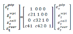
Abstract

¹Using a structural VAR model on quarterly data from 2000Q1 to 2011Q1, this paper estimated the impact of monetary policy on aggregate demand in India. The overall impact on aggregate demand is then decomposed to observe the differential impact among the various components. It finds that an interest rate hike has a significant negative impact on the growth of aggregate demand. However, the maximum impact is borne by investment demand growth and imports growth. Impact on private consumption growth and exports growth are relatively far more subdued, while there is hardly any cumulative impact on government consumption growth as it increases after some marginal fall initially. Variance decomposition analysis indicates that interest rate accounts for a significant percentage of the fluctuation in the growth of all the components of aggregate demand, except government consumption. Further, interest rate channel completely dominates exchange rate channel in monetary transmission, though the latter channel has non-negligible impact on investment and imports.

JEL: E20, E27, E52

Keywords: Monetary transmission, SVAR, impulse responses, aggregate demand components

I. Introduction

By now there seems to be a general consensus that monetary policy affects real economy at least in the short run. This has been confirmed by most of the empirical studies in the literature². However, how and through which channel monetary policy influences output and prices is still an open and unsettled issue. Different studies have emphasised the importance of various alternative channels. For instance: interest rate channel (Taylor, 1995); exchange rate channel (Obstfeld and Rogoff, 1995); asset prices (Meltzer, 1995); and credit channel (Bernanke and Gertler, 1995). An overview on the working of these various contrasting channels for better understanding of monetary policy transmission is provided in Mishkin (1995, 1996 and 2001). Further, it has been highlighted that during the recent global crisis, the importance of ‘portfolio balance channel’ and ‘expectations’ channel gained prominence (Yellen, 2011; Joyce et al. , 2011).

While the channels of monetary transmission remains a ‘black box’, given the near unanimity on its short-run impact on real economy, it is, however, important to understand as to which sectors of the economy the impact is felt the most. A given negative effect on aggregate demand or output after a monetary tightening coming from different sectors of the economy has different macroeconomic implications. Higher interest rates following monetary tightening can push the households to postpone some of their planned consumption and save more. The same higher interest rates can also make investments more costly and, therefore, temporarily slowdown investment. While both will reduce aggregate demand, the one emanating from slowdown in investment could have longer term growth implications in contrast to the one originating from decline in consumption demand. Further, net imports/exports can increase or decrease due to combined effect of exchange rate changes following as a consequence of monetary tightening and from the secondary impact of change in consumption and investment. The relative importance of these sectors in transmitting monetary policy movements can differ significantly across countries depending upon their characteristics.

In the literature, this aspect of monetary transmission to different components of aggregate demand, however, has been relatively less studied. Barran, Coudert and Mojon (1996) for the EU countries found that monetary shocks affect aggregate demand mainly through its impact on investment. Disyatat and Vongsinsirikul (2003) for Thailand also found that monetary policy operates on the real economy largely through its impact on investment. They ascribe the reason for higher interest rate leading to lower investment demand to the presence of significant bank lending channel, since investment in Thailand has historically relied heavily on bank credit.

Comparing the reaction of consumption and investments to monetary policy action in the euro area and the US, Angeloni et al. (2003) concluded that following an unexpected monetary tightening, various output components contribute to the economic slowdown by different degrees. While drop in private consumption dominated in the US, the effect on investments was more important in the euro area.

In the case of Hungary, Jakab, Varpalotai and Vonnak (2006) found that after an unexpected monetary policy tightening, drop in investments dominated the output response. They attributed the reason to higher interest rates and the slowdown of investment goods inflation, both contributing to higher user cost of capital. On the other hand, no significant change was detected in consumption and net exports.

In this study, we attempt to estimate the effect of monetary policy (change in interest rate) on various components of aggregate demand viz., private consumption, government consumption, investment, exports and imports in India. We used a structural VAR model on quarterly data from 2000Q1 to 2011Q1. The paper is organised as follows. Section II describes the methodology in brief. Section III presents the data and the results. Section IV concludes.

II. Methodology

We use a SVAR model as, unlike traditional VAR models, it can provide explicit behavioral interpretations of all the parameters.³ A standard SVAR approach involves identifying monetary policy shocks and quantifying their consequences. Within a structural VAR framework, one estimates a reduced form model which is approximated by a vector-autoregressive (VAR) specification such as,
Yt = A₁ Y_t-1 + … + A_pY_t-p + BZ_t +e_t
Where Y stands for the vector of n endogenous variables, Z contains intercept, deterministic trend and other exogenous variables, p is the number of lags included and vector e is the error term of the VAR process. A₁...A_p are nxn coefficient matrices of lagged endogenous variables and B is the matrix of coefficients of exogenous variables. After estimating the VAR model, the main task in the estimation of SVAR is to decompose residuals into structural shocks. This corresponds to finding the contemporaneous relationship between structural and reduced form innovations or finding matrix C such that
e_t = C._εt

Where e_t denotes the vector of estimated residuals and ε_t the vector of structural shocks. It is assumed that structural shocks are orthogonal to each other, while the same is not necessarily true for VAR residuals. Matrix C contains the contemporaneous impact of structural disturbances on endogenous variables. The (i,j)^th element of the structural matrix is the magnitude by which the j^th structural shock affects the i^th variable simultaneously. Since, the matrix C is not unique, which means there is more than one structural model that has the same reduced form, one has to impose additional n(n-1)/2 restrictions on C matrix in addition to n normalization to achieve full or exact identification. While working with fewer restrictions (under-identified system), the parameters we are interested in are not uniquely identified. Similarly, over identification will have more restrictions than required and the system cannot be solved. Since identification is the most sensitive part of the estimation procedure, it is desirable to use the least disputable prior knowledge about the system.

For this purpose of identification of monetary policy shock, drawing on the literature (for example, Vonnak, 2005), we use point zero restriction approach. This identification approach restricts some elements of matrix C to be zero. This strategy has the advantage that a structure of contemporaneous impacts can be translated to delayed reaction. Identification of monetary policy shocks is usually based partly on assuming no immediate effect on real variables like output and prices.

In view of the limited number of variables which can be considered in the SVAR without losing degrees of freedom, instead of examining the impact on all the components of aggregate demand at one time, they are examined separately one at a time. This involves having a benchmark SVAR model to which each of the components of aggregate demand is added each time separately to examine the impact on that component (for example, Disyatat and Vongsinsirikul, 2003; Vonnak, 2005 and Aleem, 2010).

Benchmark SVAR Model

The benchmark model is a 4-variable SVAR, consisting of output (GDP), prices (WPI), interest rate (Call rate) and real exchange rate (REER). The SVAR model with point zero restriction is as follows:

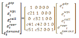
where e_t denotes VAR residual and ε_t denotes structural shocks. The first equation represents a slow response of real GDP to shocks in prices, interest rate and real exchange rate. Second equation shows that prices also respond slowly to shocks in interest rate and real exchange rate, but it reacts immediately to change in real GDP. The third equation removes the immediate effect of the shocks on output and real exchange rate on interest rate, but it reacts instantaneously to change in prices. The last equation implies that real exchange rate responds contemporaneously to shocks in real GDP and prices, but not to shocks in interest rate⁴.

The monetary transmission mechanism in the benchmark model is assessed through the impulse response function of real GDP, prices and real effective exchange rate to monetary policy shock i.e., one-standard deviation increase in policy rate.

To examine the impact of monetary policy on the components of aggregate demand, the benchmark model is augmented by including the aggregate demand components as additional variables. Given the five components of aggregate demand, thus, five augmented SVARs are estimated. The modified SVAR, using zero restriction, now takes the following form:

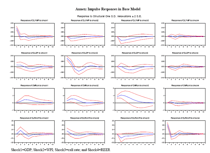
In this augmented SVAR, GDP excludes that particular component of aggregate demand which is being examined. The additional restriction in this augmented SVAR shows that a given component of aggregate demand responses contemporaneously to the remaining components of aggregate demand and prices, but reacts only slowly to interest rate and real exchange rate.

III. Data and Results

Data

All the relevant data has been obtained from Real Time Handbook of Statistics on Indian Economy, RBI. The time period covered is from 2000:Q1 to 2011:Q1. The period prior to 2000:Q1 has been excluded as interest rate was not the principal instrument of signaling policy intentions. The variables are: GDP at market prices (MP) at constant prices to capture the total aggregate demand in the economy; price is represented by WPI all commodity; policy rate is represented by weighted average call rate⁵, real exchange rate by real effective exchange rate (REER); and the various components of real GDP at MP viz., private consumption (C), investment (I), government consumption (G), exports (E) and imports (M). From GDP at MP, each components of aggregate demand was subtracted to arrive at the other residual component of aggregate demand. These are: non-investment component of aggregate demand (NIGDP); non-private consumption component of aggregate demand (NCGDP); non-export component of aggregate demand (NXGDP); non-import component of aggregate demand (NMGDP); and non-government component of aggregate demand (NGGDP)⁶. All the variables were seasonally adjusted and log transformed, except the call rate.

Results

Before the SVAR estimates, all the variables were first tested for their stationary properties. The results presented in table 1 show that, barring REER and non-government component of aggregate demand, all the remaining variables were found to be non-stationary. Thus, we formulated the SVAR in first difference form, except for the call rate.

Secondly, the appropriate lag length of the SVAR was tested. The results reported in table 2 shows conflicting results ranging from one to two lags among the five alternative tests. We, however, selected two lags as one lag was considered too short to capture the underlying dynamics.

Baseline SVAR model

As mentioned above, we begin with the performance of the benchmark model before investigating the responses of various components of aggregate demand to a monetary policy shock. Four dummy variables were used to control for extreme outliers in the residuals in each of the four variables⁷. Interestingly, inclusion of these dummy variables, by capturing the part of the overall impact of unexplained variables could also remove the problem of ‘price puzzle’.

As our focus is on the impact of policy shocks on other macro variables, we present only the impulse responses of GDP, WPI and REER to shocks in call rate in Chart 1 ^{8 9}.

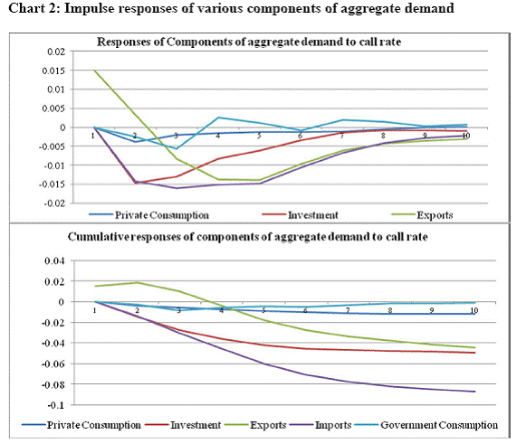
It can be observed that one standard deviation equivalent to 1.8 per cent increase in call rate reduces real GDP growth by a maximum of about 0.46 per cent below the baseline after two quarters and takes about eighth quarters to dissipate completely. The impact of monetary policy shock on inflation occurs with some lags after the impact on GDP growth. Inflation starts declining only after the second quarter and the maximum impact is felt in the fourth quarter with a decline of about 0.29 per cent below the baseline before dissipating completely by the eighth quarter.

A shock in call rate leads to depreciation in REER from the second quarter by about 0.9 per cent below the baseline before dissipating slowly. It is interesting to note that hike in call rate leads to depreciation in REER. It signifies that interest rate differentials perhaps do not play any important role in the exchange rate determination in India. This is mainly because debt component of capital flows which are sensitive interest rate differentials constitutes a small proportion of total capital flows. On the other hand, non-debt capital flows such as FDI and FII equity flows which roughly consititute three-fourth of total capital flows are insensitive to interest rate differentials (Verma and Prakash, 2011). These non-debt component of capital flows would be more strongly determined by macroeconomic fundamentals and policy environments. Thus, hike in call rate could be associated with negative sentiments about the domestic economy in terms of inflationary pressure and the dampening effect on growth, leading to slowdown in capital inflows or even outflows and, thus, to currency depreciation.

The variance decomposition in table 3 suggests that interest rate accounts for about 32.0 to 34.0 per cent of the fluctuation in real GDP growth between one to two years, with own shock accounting for over 60.0 per cent. This impact is similar to those found in the US or in some other EMEs such as Thailand, and indicates that interest rate policy has become an important determinant of fluctuations in economic activity in India¹⁰. With regard to inflation, interest rate account for about 15.0 per cent and real GDP growth for about 8.0 per cent of total fluctuation, with own shock explaining over 75.0 per cent. Inflation and real GDP growth have significant influence on interest rate accounting for about 15.0 per cent and 10.0 per cent of the total variation in call rate, respectively. On the other hand, change in real exchange rate (REER) has a very weak influence on the fluctuation of real GDP growth, inflation and interest rate. Call rate and real GDP growth, however, has a significant influence on the movement in REER accounting for about 19.0 per cent and 11.0 per cent of the total fluctuation, respectively, while the impact of inflation on change in REER is also non-negligible.

Responses of aggregate demand components

Given the result that about one-third of the fluctuation in the growth of aggregate demand (real GDP growth) is explained by shocks in policy interest rate, the next issue is to examine which of the components are most affected by monetary policy actions. For this purpose, as mentioned above, the benchmark model was augmented by each components of aggregate demand and their impulse responses to shock in interest rate were compared. Chart 2 reports the comparative impulse response of various components of aggregate demand along with the cumulative responses, which are plotted on the same scale. It can be seen that a monetary shock roughly amounting to 1.8 per cent increase in call rate has substantial differential impact on the growth of various components of aggregate demand. There is a negative impact on the growth of all the components of aggregate demand, barring the initial positive impact on exports growth which follows from depreciation in real exchange rate. The maximum negative impact is felt on investment growth and imports growth, while the impact on the growth of private and government consumption, particularly the latter, is rather very small.

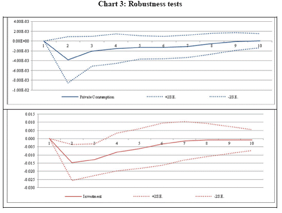
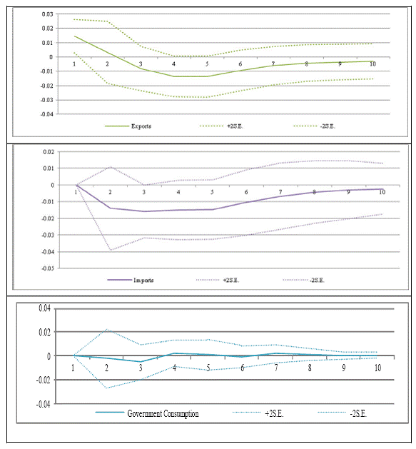
Private Consumption and Investment

The maximum impact on the growth of private consumption is only about 0.38 per cent below the base line in the second quarter and dissipates by the eighth quarter. The cumulative impact after two years is about 1.1 per cent below the baseline. In contrast, the maximum impact on investment growth, which is also felt after two quarters, is about 1.5 per cent below the baseline, roughly four times the impact on private consumption growth. The cumulative impact is about 5.0 per cent below the baseline after two years.

The variance decompositions in table 4 also show that while shock to call rate accounts for about 16 per cent of the total fluctuations in the growth of private consumption demand, it accounts for about 34.0 per cent of the total fluctuations in investment growth. Inflation and real exchange rate (about 10.0 per cent each) also have a much greater influence on investment growth than on private consumption growth (about 5.0 per cent and 2.0 per cent, respectively). Consequently, while two-third of the fluctuation in private consumption growth is explained by its own shocks, in the case of investment growth, own shocks explain only about 28.0 per cent of the total fluctuation.

In other words, it is implied that private consumption or household savings in India are less sensitive to interest rates¹¹. In this context, based on historical data, Salam et al. (2000) had found household savings in India to be less sensitive to the interest rate. Another reason for greater insensitiveness of private consumption to interest rate could be the much lower level of households’ indebtedness as compared to the developed countries. On the other hand, investment is much more sensitive to interest rate, both directly as it would raise the cost of capital and indirectly though changes in real output, price and exchange rate.

Export and Import

As explained above, hike in call rate leads to real depreciation. Initially, there is acceleration in exports growth, but it starts decelerating by the third quarter and deceleration peaks by the fifth quarter before converging back. The cumulative impact is decline in exports growth by about 4.0 per cent below the baseline growth. The impact on imports growth is much larger with a peak decline in imports growth of 1.5 per cent below the baseline growth in the fourth quarter and a cumulative decline in imports growth of about 8.5 per cent below the baseline. Variance decomposition shows that change in real exchange rate plays a more important role in explaining the fluctuations in imports growth than exports growth. While own shocks explains about 40.0 per cent of total fluctuations in exports growth, about 31.0 per cent of the total fluctuations in imports growth is explained by its own shocks. Other GDP components, inflation and interest rate have significant influences on both export and imports growth in the range of about 15.0 to 27.0 per cent after two years.

Part of the higher impact on imports growth than exports growth may be explained by the decline in investments growth, which is understood to have high import content in India. A greater decline in imports growth than exports growth would imply higher/lower net exports/imports growth, which would reduce the monetary policy impact on aggregate demand through hike in interest rate.

Government Consumption

With regard to growth in government consumption, the negative impact is seen only in the second and the third quarter, which thereafter turns mildly positive before convergence. The maximum negative impact in the third quarter is only about 0.5 per cent below the baseline and the accumulated response is almost zero. Variance decomposition shows that barring the influence of other components of aggregate demand, variation in government consumption growth is entirely self-explanatory process, indicating independence of fiscal policy from monetary policy influence.

Robustness of Results

Robustness of the results was checked by examining the statistical significance of the impulse responses. Accordingly, +/-2S.E. confidence interval was estimated for each of the impulse response function of aggregate demand components. It is seen that they are statistically significant at the conventional level in around the periods where the maximum impacts are felt for investment, exports and imports. On the other hand, they are insignificant for private consumption and government consumption throughout (Chart 3).

IV. Conclusions

Using a structural VAR model on quarterly data from 2000Q1 to 2011Q1, this paper estimated the impact of monetary policy through change in interest rate on the growth of aggregate demand. The overall impact on aggregate demand is then decomposed to observe the differential impact among the various components. It finds that an interest rate hike has a significant negative impact on the growth of aggregate demand, with the peak impact felt in the second quarter and last about eight quarters to dissipate completely. The impact on inflation follows after some lags to the impact on aggregate demand. More than one-third of the fluctuation in the growth of aggregate demand can be explained by change in interest rate, indicating interest rate has become an important determinant of fluctuations in economic activity in India.

Disaggregated analysis of the components of aggregate demand, however, shows that the maximum impact is borne by growth in investment demand and imports. Part of the impact on imports growth can be explained by the decline in investments growth, which is understood to have a high import content in India. Impact on the growth of private consumption and exports are relatively far more subdued, while there is hardly any cumulative impact on government consumption growth as it increases after some marginal fall initially. Variance decomposition analysis indicates that interest rate accounts for a significant percentage of the fluctuation in the growth of all the aggregate demand components, except government consumption. Further, interest rate channel completely dominates exchange rate channel in monetary transmission, though the latter channel has non-negligible impact on investment and imports.

^@Jeevan Kumar Khundrakpam (E-mail:) is a Director in the Monetary Policy Department.

¹These are strictly his personal views.

²Exceptions are rare such as Ulhig (2005) which could not reject neutrality of monetary policy even in the short-run.

³Both traditional VAR and SVAR, however, cannot accommodate a large number of variables without running the risk of degrees of freedom. Consequently, due to lack of sufficient variables or model misspecification, it is often found that these models suffer from ‘price puzzle’ i.e., monetary tightening initially leading to price increase, which is a contradiction to economic theory.

⁴ We followed a positive approach in our identification procedure as against based on a priori expectations derived from what ought to be theoretically. Thus, the restrictions which were either found to be statistically insignificant or led to over-identification problem were not considered.

⁵Weighted average call rate has been used as a proxy for the policy rate, as it has tended to hug the effective policy rate – repo rate or reverse repo rate – as the case may be depending upon the liquidity condition during the period under consideration.

⁶ In macroeconomics literature, even though aggregate demand and its components are generally derived from the expenditure side of national income identity, in the Indian context, we need to be cautious in using them as a proxy for demand in the economy. This follows from large discrepancies reported in the expenditure side of national accounts data, which make them not only volatile but also inconsistent in terms of national income identity itself. For instance, according to national income framework, current account balance can be alternatively defined as saving minus investment (saving-investment gap) or gross national product minus consumption minus investment minus government consumption, but Indian national accounts data would show large discrepancies between these alternative definitions.

⁷They are: DGDP = 1 for 2003:Q4 and zero otherwise; DWPI= 1 for 2000:Q3 and zero otherwise; DREER= 1 for 2007:Q4 and zero otherwise and DCall = 1 for 2007:Q1 and zero otherwise.

⁸ All the impulse responses are statistically significant at the conventional level in an around the period of peak impact.

⁹Other impulse responses are presented in the annex. We find an overall consistency in the directions of the impulse responses to our a priori expectations.

¹⁰A similar estimates including earlier period from 1996:1 to 2011:1 show that the impact of interest rate on real output is much more smaller, about 13-14 per cent only, implying increasing impact of interest rate on aggregate demand since the beginning of 2000s.

¹¹This result of monetary shocks affecting aggregate demand mainly through investment has also been found by Barran, Coudert and Mojon (1996) for the EU countries, Disyatat and Vongsinsirikul (2003) for Thailand, and Jakab et al (2006) for Hungary.

References

Aleem, Abdul [2010]. “Transmission mechanism of monetary policy in India”, Journal of Asian Economics, 21, 186-197.

Angeloni, Ignazio, Anil K. Kashyap, Benoît Mojon and Daniele Terlizzese (2003) “The output composition puzzle: a difference in the monetary transmission mechanism in the
euro area and U.S.”, Journal of Money Credit and Banking 35(6, Part 2).

Barran, F., Coudert, V., and Mojon, B. (1996), “The transmission of monetary policy in European countries”, CEPII Working Paper, February.

Bernanke, Ben and Mark Gertler (1995), “Inside the black box: the credit channel of monetary transmission”, Journal of Economic Perspectives, 9, 27-48.

Disyatat, Piti and Pinnarat Vongsinsirikul (2003), “Monetary policy and the transmission mechanism in Thailand”, Journal of Asian Economics, 14.

Jakab, Varpalotai and Vonnak (2006) “How does monetary policy affect aggregate demand? A multimodel approach for Hungary”, Magyar Nemzeti Bank WP 2006/4.

Joyce, Michael; Matthew Tong and Robert Woods (2011), “The United Kingdom’s quantitative easing policy: design, operation and impact”, Quarterly Bulletin 2011 Q3, Bank of England.

Meltzer, Allan H. (1995), “Monetary, credit and (other) transmission processes: a monetarist perspective,” Journal of Economic Perspectives, 9, 49-72.

Mishkin, Frederic S. (1995), “Symposium on the monetary transmission mechanism”, Journal of Economic Perspectives, 9, 3-10.

Mishkin, Frederic S. (1996), “Channels of monetary transmission and lessons for monetary policy”, NBER Working Paper No.5464, National Bureau of Economic Research.

Mishkin, Frederic S. (2001), “The transmission mechanism and the role of asset prices in monetary policy”, NBER Working paper No.8617, National Bureau of Economic Research.

Obstfeld, Maurice and Kenneth Rogoff (1995). “The mirage of fixed exchange rates”, Journal of Economic Perspectives, 9, 73-96.

Taylor, John B. (1995), “The monetary transmission mechanism: an empirical framework”, Journal of Economic Perspective, 9, 11-26.

Salam, A. and U. Kulsum (2000) Savings behavior in India: An empirical Study, Department of Economics, AMU, Aligarh.

Trichet, Jean-Claude (2011), Introductory statement to the press conference, European Central Bank, Frankfurt, February 3.

Uhlig, Harald (2005), “What Are the Effects of Monetary Policy on Output? Results from
an Agnostic Identification Procedure”, Journal of Monetary Economics, 52.

(Verma and Prakash, 2011), “Sensitivity of Capital Flows to Interest Rate Differentials: An Empirical Assessment for India”, RBI Working Paper, WPS (DEPR): 7/2011, May.

Vonnák, Balázs (2005) “Estimating the Effect of Hungarian Monetary Policy within a Structural VAR Framework”. MNB Working Paper No. 2005/1.

Yellen, Janet L. (2011). “Unconventional monetary policy and central bank communication” Speech at the University of Chicago Booth School of Business U.S. Monetary Policy Forum, New York, New York, February 25.