Sujata Kundu, Anshu Kumari and Deepika Rawat^*

Received: November 3, 2022
Accepted: January 11, 2024

The paper studies the evolving dynamics in cross-border capital flows, with an emphasis on the emerging market economies (EMEs) covering a timeline of three decades (Q1:1992-Q1:2022). In view of the persistent volatility in capital flows to EMEs, the paper examines major episodes of capital flow reversals, in particular sudden stops. The empirical analysis suggests that global factors – global growth, risk, liquidity, long-term interest rates, policy rate changes – along with domestic growth and nominal exchange rate dynamics are key drivers of capital flow reversal episodes in the EMEs. The appropriate utilisation of capital flow management measures (CFMs) and macroprudential policy measures (MPMs), along with a strengthening of domestic macroeconomic and financial fundamentals and adequate buffers in the form of foreign exchange reserves, can help the EMEs navigate the ebbs and surges in capital flows better, while preserving macroeconomic and financial stability.

JEL Classification: F3, F32, F320, F41

Keywords: Capital flows, capital flow reversal, cloglog model, foreign portfolio investment, gross capital inflows, monetary policy communication, net capital flows, sudden stop, taper tantrum.

Introduction

International capital mobility has witnessed a significant surge since the early-1990s, led by both country-specific and global developments. While domestic pull factors, such as structural reforms, capital account liberalisation and stabilisation programmes in several emerging market economies (EMEs) improved creditworthiness, drove productivity gains and investors’ confidence in macroeconomic management, global push forces, such as the decline in real interest rates in the advanced economies (AEs) in the early-1990s also attracted foreign investors towards EMEs. Further, global easing in communication costs and increased competition led firms in AEs to locate their production centres in EMEs to garner production efficiency and profits. Moreover, as EMEs gradually moved towards capital account liberalisation, institutional investors discovered wider opportunities in EMEs for risk diversification. Consequently, the volume of capital flowing into EMEs rose, simultaneously resulting in risks of sudden shifts and reversals in capital flows and increased financial market volatility.

From the standpoint of the EMEs, cross-border capital flows help in the mobilisation of external savings, which has been perhaps the strongest argument in favour of international capital mobility (Devlin et al., 1994). While from a macroeconomic perspective, net inflows of external savings supplement domestic savings, from the financial stability angle, gross capital flows provide insights into the international exposure of an economy (Lane and Milesi-Ferretti, 2007; Tarashev et al., 2016; OECD, 2018). Spillovers and contagions are often transmitted and amplified across economies via the channel of gross capital flows (BIS, 2021). Therefore, their impact is wide-ranging, affecting an array of macroeconomic parameters, including exchange rates, interest rates and foreign exchange reserves. Large capital inflows/ reversals are often associated with macroeconomic and financial sector disruptions (Calvo et al., 1993; Kamin and Wood, 1997; Lopez-Mejia, 1999; Kohli, 2001)¹.

The period since the 1990s has been eventful, characterised by extraordinary movements in global capital flows, not only in terms of their levels but also volatility along with extreme movements or capital flow “waves”². After surging through the mid-2000s, capital flows contracted during the Global Financial Crisis (GFC) of 2008-09. An array of global events including highly accommodative monetary policies by the major AEs with policy rates close to zero or even negative (both after the GFC and the COVID-19 pandemic), the taper tantrum of 2013-14, Chinese stock market sell-off, the devaluation of the Chinese renminbi, the outbreak of COVID-19 in 2020, monetary policy normalisation by major AE central banks beginning 2021 and the Russia-Ukraine war in 2022 have imparted sizeable volatility to capital flowing into EMEs. Surges in capital flows and sudden stops³ have significant adverse effects on the EMEs. Capital flow reversals are generally sudden, large, disruptive and broad-based with a limited window for policy reactions. As capital flows often obey global factors and events, there is a need for policy preparedness and a careful monitoring of domestic and global macroeconomic conditions.

Set against this background, this paper has two objectives. First, it attempts to study the evolving dynamics in global capital flows during the post-GFC period, with a focus on the EMEs. The paper provides an account of the major episodes of sudden stops for a sample of major EMEs, covering a period of 30 years (Q1:1992 to Q1:2022). Secondly, it examines the key drivers of such reversal episodes. The paper is structured as follows: Section II presents a review of the literature on identifying episodes of sudden stops in EMEs. Section III provides the stylised facts on capital flow developments globally and in India since the 1990s. Section IV discusses the empirical findings related to the identification and drivers of major episodes of capital flow reversals, distinguishing them from sudden stops. Section V concludes the paper.

Section II
Literature Review

Following Calvo (1998), the balance of payments (BoP) accounting identity after subtracting errors and omissions rests on the following equation:

where, KI, CAD and RA represent capital inflows, current account deficit and accumulation of international reserves, respectively. When a sudden stop occurs causing the financial account (FA) of the BoP to shift towards outflows, the current account (CA) balance has to improve (implying CAD in identity (1) must fall quickly and sizeably and transit towards a surplus), assuming central banks do not intervene through the sale of international reserves [RA in identity (1)]. The fall in CAD may happen either through a rise in domestic savings or a fall in investment⁵. Such adjustment usually accompanies a cyclical slowdown, or a recession, with a related significant decline in national income. BoP crises are usually characterised by such type of adjustments (Cecchetti and Schoenholtz, 2018).

A series of EME crises in the 1990s⁶ increased the academic and policy interest in sudden stops, which were spelt out as a phase of an abrupt reversal in net flows. During such episodes, the associated adjustments in CA balance and RER depreciation often resulted in significant loss of output in the crisis economies (Calvo, 1998; Calvo et al., 2004, 2008). In contrast to the 1990s, when net capital flows closely mimicked gross capital inflows, especially in the context of EMEs, gross inflows and outflows have surged since the early-2000s in terms of both level and volatility, weakening the relationship between gross and net inflows. Domestic and foreign investors often react differently to various shocks and policy measures/responses need to consider the sources of extreme movements in capital flows, i.e., whether driven by foreign investors (surges or sudden stops) or domestic investors (capital flight or retrenchment). Therefore, the recent literature on sudden stops has taken into account gross inflows instead of net flows to identify and analyse such episodes (Cowan and De Gregorio, 2007; Agosin and Huaita, 2011; Forbes and Warnock, 2012; Eichengreen and Gupta, 2016; Forbes and Warnock, 2021).

Following the taper tantrum of 2013 and the accompanying significant capital flow reversals, more financially developed EMEs with more liquid capital markets and higher inflows recorded larger pressure on their exchange rates, foreign reserves, and equity prices (Aizenman, Binici and Hutchison, 2014; Eichengreen and Gupta, 2015). Annex Table A1 provides a broad summary of the available literature on sudden stop episodes, in both AEs and EMEs, including major studies that examined the impact of the taper tantrum on EMEs.

Section III
Salient Stylised Facts

Following a surge through the mid-2000s, capital flows contracted during the GFC. In the post-GFC period, beginning around 2010, capital flows recovered, driven by highly accommodative monetary policies and large-scale asset purchases by the major AE central banks. Capital flows declined during 2013-15 on the back of the US Federal Reserve’s (Fed’s) announcement of its intention towards monetary policy normalisation and tapering its asset purchase programme. In particular, foreign portfolio investment (FPI) flows reversed from the EMEs. The Chinese stock market sell-off and the devaluation of Renminbi also contributed to the moderation in capital flows. In 2020, with the outbreak of the COVID-19 pandemic, capital flows again recorded exceptionally large swings, especially in the initial months. FPI flows to EMEs reversed with unparalleled speed and magnitude amidst extreme uncertainty and flight to safety. With central banks in the major AEs shifting to extremely accommodative monetary policies – including sharp cuts in policy rates and large asset purchases – capital flows to EMEs revived in late-2020 and 2021.

In 2021, inflation recorded decadal highs both in the AEs and EMEs owing to supply chain disruptions induced by the pandemic, heightened commodity price pressures due to geopolitical tensions, and strong demand recovery. With inflation well above target, major AE central banks were forced to pursue an aggressive synchronised monetary policy normalisation in 2022. As a result, during 2022, EMEs faced intense financial market volatility, short-term portfolio capital outflows, foreign exchange reserve losses and currency depreciation pressures.

III.1 Movements in Global Capital Flows

In the case of foreign direct investment (FDI) flows, EMEs showed some recovery in the post-GFC period and the trend remained largely stable till the outbreak of the pandemic in 2020 (Chart 1a). There was a drop in net FPI flows in 2015 (Chart 1b). The volume to EMEs did not increase significantly during 2016-21; it remained slightly lower as compared to the six-year period from 2009-14 prior to the drop in 2015.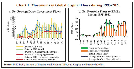

Volatility in both FDI and FPI flows to EMEs dropped in the post-GFC period (Charts 2a and 2b), with this period being characterised as “great moderation” in the volatility of capital flows, in particular to the EMEs (McQuade and Schmitz, 2017; Pagliari and Hannan, 2017). However, volatility in both net FDI and FPI flows has increased since 2020, particularly for the EMEs.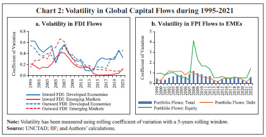

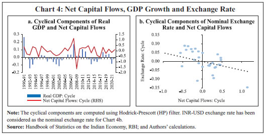
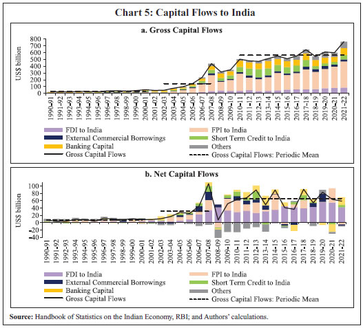
III.2 Trends in India

India, in line with the global trends, saw a steady increase in capital flows following the structural reforms, including capital account liberalisation, in the early-1990s (Chart 3a). Foreign investment responded favourably over the years with FDI and FPI flows emerging as the important sources of external finance and non-debt flows exceeding debt flows in the form of non-resident deposits, external commercial borrowings and external assistance. India witnessed an upsurge in net capital flows from 2003-04 until the GFC. In terms of annual averages, net capital flows were around US$ 31.3 billion during 2000-01 to 2007-08 as compared to US$ 7.7 billion during 1990-91 to 1999-2000.

A sudden stop in capital inflows occurred during the GFC⁷, after which the inflows showed a recovery. The subsequent years recorded a substantial increase in net capital flows averaging around US$ 67.9 billion per annum during 2010-11 to 2021-22. The overall volatility in net capital flows to India declined in the post-GFC period (Chart 3b).

Capital flow liberalisation has led to a greater financial integration of India with the global economy. In tandem with the other EMEs, and as indicated in the literature, net capital flows to India have been procyclical i.e., in times of higher economic growth, net capital flows have also generally remained higher and vice versa and have reflected in exchange rate appreciation (depreciation) (Chart 4). Component-wise, while gross capital flows have been dominated by FPI, in net terms FDI to India has risen over the years (Chart 5).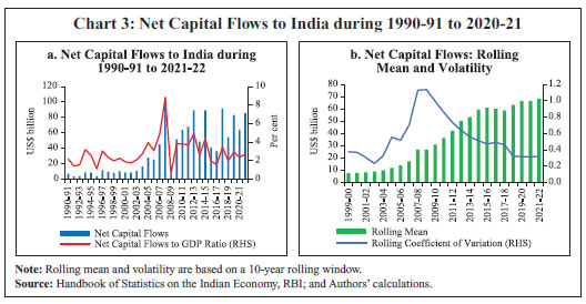

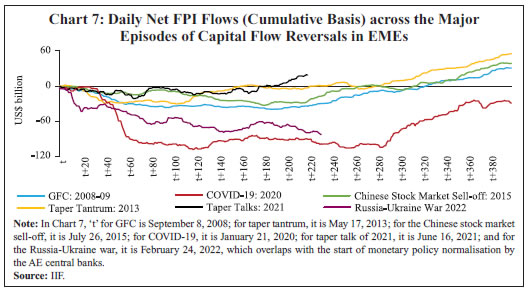
Section IV
Capital Flows and Sudden Stops: An Empirical Analysis

As indicated earlier, capital flows to EMEs have generally been volatile, with various components exhibiting significant differences in the levels of volatility. For example, FPI flows have shown higher volatility as compared with FDI flows (Chart 6). Further, Chart 7 highlights the magnitude and intensity of reversals in net FPI flows from EMEs during the major shock episodes in the past two decades since the GFC. It indicates that the volatility experienced by EMEs in FPI flows since the COVID-19 outbreak has been significantly higher than the GFC as well as the 2013 taper episode.

Against this background, this section provides an account of the sudden stop episodes in EMEs during the previous three decades. It considers a sample of 19 economies, including India, covering a span of about 30 years (Q1:1992 to Q1:2022). It then focuses on India and the set of EMEs to analyse the key driving factors behind the capital flow reversal episodes.

IV.1 Identifying Episodes of Capital Flow Reversals in EMEs

(a) Event Study Framework

To begin with, the paper first considers the past two decades (2001-2022) marked by a major surge in EME capital inflows. As discussed earlier, the scale of the impact of the shocks on net FPI flows has varied widely, not only in terms of the level, but also with respect to the duration taken for the correction in flow reversals (Chart 7). Therefore, as a first step towards identifying the severity of these episodes in terms of their impact on net FPI flows⁸, a panel data-based event study approach is adopted using the weekly FPI net flows data⁹ for 10 major EMEs plus South Korea¹⁰. The period of analysis differs across the episodes¹¹. The approach has gained popularity in recent years and has been used to analyse the impact of the pandemic on various macroeconomic parameters (Mishra et al., 2014).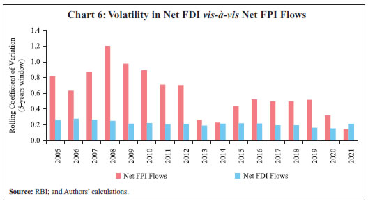

The following equation is used to examine the impact of the various episodes on the weekly net FPI flows in the EMEs: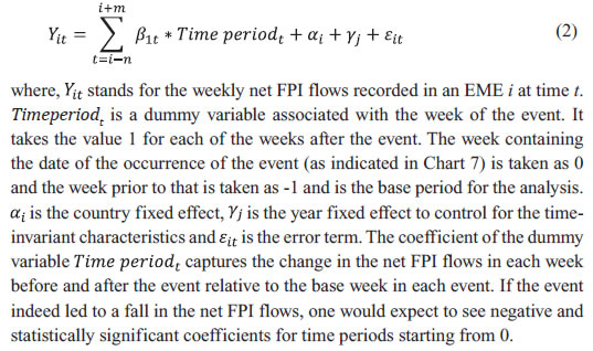

The results show that weekly net FPI flows to the EMEs were heavily impacted during the GFC, the taper tantrum episode of 2013, the COVID-19 pandemic, the Russia-Ukraine war and the synchronised aggressive monetary tightening by AEs in 2022 (Chart 8)¹². The Chinese stock market sell-off event during 2016 did not produce any statistically significant decline in overall net FPI flows to the EMEs (Chart 8c). In terms of the statistical significance, the immediate impact of the pandemic and GFC were much stronger as indicated by the narrower confidence bands around the estimated coefficients (Charts 8a and 8d). Moreover, the impact of the pandemic persisted longer as compared with the other episodes. Further, the multiple waves of the pandemic also had an adverse effect.

In contrast to 2013, the taper talks of 2021 did not create any major impact on the net FPI flows to the EMEs. While net flows declined significantly in some weeks of 2021 as the taper talks began (with the actual tapering starting only in November 2021), the impact was broadly contained. The statistically significant dip in net FPI flows around t = 18 to 25 (Chart 8e) is the period around which the US Fed began its actual tapering of asset purchases during November 2021. The weak impact could perhaps be due to the fact that the US Fed was still making large asset purchases of US$ 105 billion per month in November 2021 as compared with US$ 120 billion in the previous month. Moreover, the macroeconomic fundamentals of the EMEs had strengthened sizeably relative to 2013.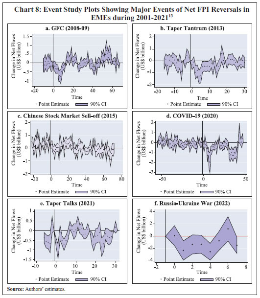

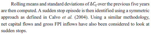
While the event study framework provides a comparison of the severity of the episodes in terms of the magnitude and duration of the impact, not all of these episodes can qualify as sudden stops. Therefore, as a second step to the analysis, the definition provided by Calvo et al. (2004) has been followed to identify the sudden stop episodes.

(b) Calvo et al. (2004) Methodology for Identifying Sudden Stops

According to Calvo et al. (2004), a sudden stop is a phase that satisfies the following criteria: (i) it contains at least one observation where the year-on-year (y-o-y) decline in capital flows falls at least by two standard deviations below its sample mean; and (ii) the phase ends once the annual change in capital flows exceeds one standard deviation below its sample mean; and (iii) for symmetry, the start of a sudden stop phase is determined by the first time the annual change in capital flows falls one standard deviation below the mean. This implies that a sudden stop episode starts with a fall in capital flows exceeding one standard deviation below the mean, followed by a fall of two standard deviations and the process lasts until the change in capital flows moves above mean minus one standard deviation. Given this definition and the growing importance of gross capital flows in the post-GFC years as indicated in the previous sections, the sudden stops have been identified in this section on the basis of gross capital inflows using the methodology adopted by Forbes and Warnock (2012) [similar methodology is also given in Cavallo et al. (2015)].

Quarterly data on gross inflows and net flows for a sample of 19 EMEs (including South Korea)¹⁴ over the period Q1:1992 to Q1:2022 as available in the Balance of Payments Statistics (BOPS) of the IMF have been used for the purpose. Given below is the detailed methodology used for the identification of sudden stops: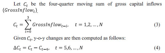

The results indicate that, for the sample of all EMEs, GFC is the only sudden stop episode during Q1:1992 to Q1:2022 both in terms of gross capital inflows and net flows (Chart 9). However, in EMEs excluding China, the pandemic quarters of Q3 and Q4:2020 have also been identified as sudden stop phases, albeit on the basis of net capital flows only (Chart 9d).

A disaggregated country-level analysis reveals that sudden stops were recorded in some EMEs, such as Brazil, China, Colombia, India, Indonesia, South Korea, Mexico and Sri Lanka during H2:2015 and H1:2016. These were a result of the international financial market turmoil in August 2015 due to the Chinese stock market sell-off and the first hike in the US Federal Funds rate in December 2015 after a long pause (Annex Table A2). Interestingly, none of the taper talk episodes, either the taper tantrum phase of 2013 or the taper talks of 2021, were identified as sudden stops¹⁵. These findings are in line with the existing literature (Gupta, 2016; Eichengreen and Gupta, 2016; Forbes and Warnock, 2021)¹⁶.

As FPI flows have higher volatility and are more often impacted by global shocks, the same analysis was repeated considering gross FPI inflows for the same set of EMEs and sample period. The results were unchanged at the aggregate level. At a disaggregated level, EMEs that witnessed sudden stops during the taper talks and/or the beginning of taper during 2013 and 2014 were Türkiye (Q4:2013 to Q2:2014), Mexico (Q4:2013), Thailand and Ukraine (Q1:2014)¹⁷. Both China and India recorded sudden stops during Q1:2022 with respect to gross FPI inflows.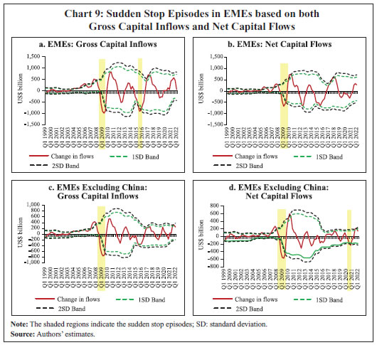

IV.2 Factors Driving Capital Flow Reversals

The literature provides an array of factors that drive global capital flow waves, mainly classified into “push” factors – forces driving capital flows external to the domestic economy and “pull” factors – forces relating to the domestic economy that help in attracting capital flows. Some of the seminal papers in this area of work, such as Calvo et al. (1993, 1996), Fernandez-Arias (1996), and Chuhan et al. (1998) find push factors to be more significant than pull factors in driving capital flows, although Calvo et al. (1996) highlight that better domestic policies and economic performance had initially contributed to the surge in capital inflows to EMEs. However, subsequently, global factors became more important, especially the movements in global interest rates.

In this paper, following Forbes and Warnock (2012, 2021), the major factors driving capital flow reversal episodes have been identified for the 19 EMEs (as defined in the previous sub-section) during Q1:1992 to Q1:2022. Annex Table A4 provides the details of the variables/ indicators that have been used for the empirical analysis. The variables have been identified based on the review of the extant literature. In order to examine the role played by these variables in the conditional probability of having an episode of capital flow reversal each quarter, the model estimated is as follows: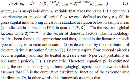

The results presented in Table 1 for India indicate weak global economic growth, higher global interest rates and higher global risk as crucial factors associated with a fall in gross capital inflows. The y-o-y increases in long-term global interest rates as well as the US Federal Funds rate raise the likelihood of capital flow reversals, which is in sync with our expectations. Exchange rate depreciation also increases the probability of capital flow reversals. Domestic macroeconomic variables, such as GDP growth and inflation are not found to be statistically significant. In an extended analysis, global liquidity and domestic CAD also turn out to be significant drivers of gross capital flows, wherein a rise in global liquidity lowers the likelihood of a capital flow reversal episode, while a rise in the CAD raises its likelihood (Annex Table A5.3). Overall, the results point to the significant role played by global factors in capital flow reversal episodes in India, consistent with the extant cross-country literature (Albuquerque et al., 2005; Bacchetta and van Wincoop, 2010; Gourio et al., 2010; Forbes and Warnock 2012, 2021).

Moving on to the EME panel, the results suggest that, among the global factors, global risk, global liquidity, crude oil prices and policy rate differentials with the US Federal Funds Rate are statistically significant in predicting capital flow reversals. Amongst domestic factors, real GDP growth, exchange rate movements and domestic monetary policy rate are important drivers of sudden stops (Table 2). Sound macroeconomic fundamentals mitigate the probability of capital flow reversals to external shocks. For instance, during the taper talks of 2013, weak economic growth prospects coupled with high current account deficits and elevated inflation contributed towards adverse investor sentiments and EME portfolio outflows (Sahay et al., 2014; Mishra et al., 2014; Eichengreen et al., 2022)²⁰.

Section V
Conclusion

Cross-border capital mobility has witnessed a significant surge since the early-2000s led by both country-specific and global developments. While large capital inflows can contribute to higher domestic investment and growth, they remain quite volatile. Sudden reversals in capital flows can lead to increased financial market and macroeconomic volatility. This paper identified the major episodes of capital flow reversals or sudden stops for a sample of major EMEs covering a span of three decades (1992-2022). It also analysed the major drivers of capital flow reversal episodes.

The analysis indicated that the volatility in capital flows moderated post-GFC, albeit with some increase after the outbreak of the pandemic in 2020. In terms of the statistical criteria following Calvo et al. (2004), the GFC was the only major sudden stop episode for EMEs both in terms of gross capital inflows and net capital flows. The pandemic quarters of Q3 and Q4:2020 were sudden stop phases in terms of net capital flows. Global factors (global growth, global risk, US Federal Funds rate and global liquidity) as well as domestic growth predicted capital flow reversal episodes for the sample EMEs.

Capital flow reversals are generally sudden, disruptive and broad-based with a limited window for policy reaction and can lead to large volatility in domestic financial market conditions and have an adverse impact on inflation and output. The appropriate utilisation of CFMs and MPMs, along with a strengthening of domestic macroeconomic and financial fundamentals and adequate buffers in the form of foreign exchange reserves, can help the EMEs better navigate the ebbs and surges in capital flows while preserving macroeconomic and financial stability.

References

Agosin, M.R., & Huaita, F. (2011). Capital flows to emerging economies: Minsky in the tropics. Cambridge journal of economics, 35(4), 663-683.

Aizenman, J., Binici, M., & Hutchison, M.M. (2014). The transmission of Federal Reserve tapering news to emerging financial markets (No. w19980). National Bureau of Economic Research.

Albuquerque, R., Loayza, N., & S., Luis. (2005). World market integration through the lens of foreign direct investors. Journal of International Economics. 66(2), 267–295.

Bacchetta, P., & Wincoop, E.V. (2010). On the global spread of risk panics. Mimeo. Paper presented at European Central Bank conference, “What Future for Financial Globalization” on 09/09/10.

BIS (2021). Changing patterns of capital flows. CGFS Papers No. 66. May.

Broner, F., & Rigobón, R. (2004). Why are capital flows so much more volatile in emerging than in developed countries? Available at SSRN 884381.

Calvo, G.A., Leiderman, L., & Reinhart, C.M. (1993). Capital inflows and real exchange rate appreciation in Latin America: The role of external factors. IMF Staff Papers, 40(1), 108-151.

Calvo, G.A., Leiderman, L., & Reinhart, C.M. (1996). Inflows of capital to developing countries in the 1990s. Journal of Economic Perspectives, 10(2), 123-139.

Calvo, G.A. (1998). Capital flows and capital-market crises: The simple economics of sudden stops. Journal of Applied Economics, 1(1), 35-54.

Calvo, G.A., Izquierdo, A., & Mejia, L.F. (2004). On the empirics of sudden stops: The relevance of balance-sheet effects. NBER Working Paper 10520.

Calvo, G.A., Izquierdo, A., & Mejía, L.F. (2008). Systemic sudden stops: The relevance of balance-sheet effects and financial integration (No. w14026). National Bureau of Economic Research.

Cavallo, E. A. (2019). International capital flow reversals (No. IDB-WP- 1040). IDB Working Paper Series.

Cavallo, E., Powell, A., Pedemonte, M., & Tavella, P. (2015). A new taxonomy of sudden stops: Which sudden stops should countries be most concerned about? Journal of International Money and Finance, 51, 47-70.

Cecchetti, S. & Schoenholtz K. (2018). Sudden stops: A primer on balance-of-payments crises. First posted on: Money and Banking, 25 June 2018.

Chuhan, P., Claessens, S., & Mamingi, N. (1998). Equity and bond flows to Latin America and Asia: The role of global and country factors. Journal of Development Economics, 55(2), 439-463.

Cowan, K., & De Gregorio, J. (2007). International borrowing, capital controls, and the exchange rate: Lessons from Chile. In Capital Controls and Capital Flows in Emerging Economies: Policies, Practices, and Consequences (pp. 241-296). University of Chicago Press.

Devlin, R., Ffrench-Davis, R., & Griffith-Jones, S. (1994). Surges in capital flows and development: An overview of policy issues.

Eichengreen, B., & Gupta, P. (2015). Tapering talk: The impact of expectations of reduced Federal Reserve security purchases on emerging markets. Emerging Markets Review, 25, 1-15.

Eichengreen, B., & Gupta, P. (2016). Managing sudden stops. World Bank Policy Research Working Paper, (7639).

Eichengreen, B., Gupta, P., & Choudhary, R. (2022). The taper this time. Indian Public Policy Review, Vol. 3 (1).

Fernandez-Arias, E. (1996). The new wave of private capital inflows: Push or pull? Journal of Development Economics, 48(2), 389-418.

Forbes, K.J., & Warnock, F.E. (2012). Capital flow waves: Surges, stops, flight, and retrenchment. Journal of international economics, 88(2), 235-251.

Forbes, K.J., & Warnock, F.E. (2021). Capital flow waves–or ripples? Extreme capital flow movements since the crisis. Journal of International Money and Finance, 116, 102394.

Gourio, F., Michael S., & Adrien V. (2010). International risk cycles. Mimeo. Paper presented at European Central Bank conference, What Future for Financial Globalization on 09/09/10.

Gupta, P. (2016). Capital flows and central banking: The Indian experience. In Monetary Policy in India (pp. 385-424). Springer, New Delhi.

Joyce, J.P., & Nabar, M. (2009). Sudden stops, banking crises and investment collapses in emerging markets. Journal of Development Economics, 90(2), 314-322.

Kamin, S. B., & Wood, P. R. (1997). Capital inflows, financial intermediation, and aggregate demand: Empirical evidence from Mexico and other Pacific Basin countries. Board of Govs of the Fed Reserve System Internat’l Finance Paper, 583.

Koepke, R., & Paetzold, S. (2020). Capital flow data–A guide for empirical analysis and real-time tracking. IMF Working Paper WP/20/171.Kohli, R. (2001). Capital flows and their macroeconomic effects in India. IMF Working Paper, WP/01/192.

Kohli, R. (2001). Capital flows and their macroeconomic effects in India. IMF Working Paper No. 2001/192.

Lane, P.R., & Milesi-Ferretti, G.M. (2007). The external wealth of nations mark II: Revised and extended estimates of foreign assets and liabilities, 1970–2004. Journal of international Economics, 73(2), 223-250.

Lopez-Mejia, A. (1999). Large capital flows: A survey of the causes, consequences, and policy responses. Finance and Development. September.

McQuade, P., & Schmitz, M. (2017). The great moderation in international capital flows: A global phenomenon? Journal of International Money and Finance, 73, 188-212.

Mishra, M. P., Moriyama, M. K., N’Diaye, P. M. B., & Nguyen, L. (2014). Impact of Fed tapering announcements on emerging markets. International Monetary Fund.

OECD (2018). Review of the OECD code of liberalisation of capital movements - Measurement and Identification of Capital Inflow Surges. September.

Pagliari, M.S., & Hannan, S.A. (2017). The volatility of capital flows in emerging markets: Measures and determinants. International Monetary Fund.

Sahay, M.R., Arora, M.V.B., Arvanitis, M.A.V., Faruqee, M.H., N’Diaye, M.P., & Griffoli, M.T.M. (2014). Emerging market volatility: Lessons from the taper tantrum. IMF Staff Discussion Note 14/09.

Strauss-Kahn M. (2020). Can we compare the COVID-19 and 2008 crises? New Atlanticist (May 5), Atlantic Council.

Tarashev, N., Tsatsaronis, K., & Borio, C. (2016). Risk attribution using the shapley value: Methodology and policy applications. Review of Finance, 20(3), 1189-1213.

Annex

^* Sujata Kundu is Assistant Adviser, and Anshu Kumari and Deepika Rawat are Managers in the Department of Economic and Policy Research, Reserve Bank of India. Corresponding author email address: skundu@rbi.org.in. The authors are thankful to Rajeev Jain, Vidya Kamate and an anonymous referee for their valuable comments and suggestions on the paper. The views expressed in the paper are those of the authors and do not represent the views of the institution they are affiliated with.

¹ An unwarranted expansion in aggregate demand owing to excessive capital inflows (macroeconomic overheating) could be reflected in higher inflation, real exchange rate (RER) appreciation and higher current account deficit along with its sustainability issues. Moreover, the accumulation of international reserves by central banks, unless sterilised, could lead to more than desired increases in money supply, thus adversely impacting domestic price and financial sector stability. On the other hand, reversal episodes are often associated with macroeconomic and financial sector instability due to large exchange rate depreciation, high inflation, interest rate hikes and output losses, depletion of foreign exchange reserves, and stress in the corporate and banking sectors.

² Comprising episodes of ‘surges’ or ‘bonanzas’, ‘capital flight’, ‘retrenchment’ and ‘sudden stops’ (Forbes and Warnock, 2012).

³ These are episodes that witness sharp contractions in international capital flows as against capital flow surges.

⁴ In a non-monetary economy, RA is absent.

⁵ Y = C + I + G + NX, where Y, C, I, G and NX (X-M) represent aggregate demand, consumption, investment, government expenditure and balance of goods and services in the BoP, respectively. Current account balance (CAB) = NX + net income from abroad (NY) + net current transfers (NCT). Gross national disposable income (GNDY) = C + I + G + CAB, or GNDY – C – G = S = I + CAB; or, S – I = CAB.

⁶ Including the Mexican crisis (1994), Argentinian crisis (1995), the Asian crisis (1997), the Russian crisis (1998) and the Brazilian crisis (1999).

⁷ Literature has identified the crisis year of 2008-09 as a year of sudden stop in capital inflows (Gupta, 2016).

⁸ FPI constitutes only one component of the total capital flows in EMEs. Being short-term in nature and highly volatile, FPI flows are often considered to analyse capital flow reversals in EMEs. The literature suggests that median volatility is greater in the case of portfolio flows than other types of capital flows (Pagliari and Hannan, 2017). Moreover, the availability of high frequency net FPI flows data across EMEs makes it easier to use these data for an event study analysis.

⁹ Sourced from the Institute of International Finance (IIF).

¹⁰ The EMEs include India, Indonesia, Thailand, South Africa, Hungary, Türkiye, Mexico, Poland, Brazil, and Philippines. South Korea has also been included in the panel as it joined the ranks of a developed country only in 1996 following its membership in the OECD. As per the IMF’s/World Bank’s classifications, South Korea became an advanced economy/high-income country in 1997 and 2001, respectively. Moreover, South Korea is part of the MSCI Emerging Markets Index and the South Korean Won trades as a non-deliverable currency. Broner and Rigobón (2004) showed that EME capital flows have higher volatility as compared to that of AEs.

¹¹ The period of analysis for the different episodes is as follows: GFC - January 2007 to December 2009; taper tantrum 2013 - January 2012 to December 2013; Chinese stock market sell-off - January 2014 to December 2016; COVID-19 - January 2019 to December 2020; taper talks 2021 - January 2021 to January 2022; and Russia-Ukraine War - February 2022 to October 2022.

¹² As only a few data points are available for this plot, the time period is taken from January 2021 to September 2022 as per data availability.

¹³ Annex Table A3 provides the basic statistics with regard to the key macroeconomic indicators during these episodes.

¹⁴ The major EMEs that were considered for the sudden stop analysis were: Brazil, Russia, India, China, South Africa, Indonesia, Malaysia, Philippines, Thailand, Vietnam, Colombia, Mexico, Hungary, Poland, Türkiye, Ukraine, Pakistan, Sri Lanka, and South Korea. The EMEs were selected based on adequate time series data availability on capital flows in the BoP Statistics of IMF’s International Financial Statistics (IFS).

¹⁵ Similar exercise was also repeated using a shorter period of 3 years for the computation of rolling mean and standard deviation of change in gross FPI inflows. The results remained unaltered.

¹⁶ For instance, Eichengreen and Gupta (2016), while extending their analysis on sudden stop episodes in EMEs using data during 1991 to 2014, concluded that the frequency and duration of sudden stops remained largely unchanged since 2002. With regard to the taper tantrum episode of 2013, their study indicated that the period recorded smaller reversals in capital flows and had a milder impact on key macroeconomic indicators. The study referred to the episode as a ‘sudden pause’ instead of a sudden stop in capital flows. In another study, Forbes and Warnock (2021) stated, “Since the GFC, capital flows have moved more in ‘‘ripples” rather than ‘‘waves”.”

¹⁷ It is important to discuss the nature of the shock. For instance, the GFC in 2008-09 was an endogenous financial shock that affected the demand-side first and then led to the Great Recession of 2009 (Strauss-Kahn, 2020). The initial financial shock resulted in a burst of the housing bubble in the US and, hence, of demand via wealth effects. Both affected economic activity in the US and international financial markets, leading progressively to a global recession. Therefore, all actions were aimed at reviving the financial sector to lift up the economy. On the other hand, the pandemic was an exogenous shock (health emergency) and affected first the real sector and the supply-side dynamics followed by its impact on the financial sector and the demand-side. In 2008, insufficiently capitalised banks were a part of the problem. However, over the years, financial sector regulation has improved. Also, drawing insights from the previous crisis episodes, central banks were faster to react. During taper tantrum of 2013-14, central banks responded to the exchange market pressure by foreign exchange market interventions, allowing freer movement of exchange rates, changing domestic interest rates and imposing capital controls. Moreover, in the post-GFC period, countries had also built up their foreign exchange reserve buffers.

¹⁸ For the purpose of the empirical analysis in this section, a weaker definition of sudden stops has been used.

¹⁹ Unit root test results are provided in Annex Table A5.1.

²⁰ Other variables, such as domestic CPI inflation, global long-term interest rate and US Federal Funds rate were also used in alternate model specifications. However, they did not turn out to be statistically significant.

²¹ Dummy for gross capital flow sudden stop has 1674 observations, out of which 154 are non-zero outcomes. Dummy for gross FPI-based sudden stop has 177 non-zero outcomes. Among the 19 economies for which sudden stops were calculated, 18 were selected for the panel regression. Pakistan was dropped due to data comparability issues. The panel clog-log model uses random effects. To test if the random effect is suitable for the data, Hausman test was carried out for model (1). The test suggested random effect with chi2(5) = 3.02 to be statistically not significant (p-value 0.70). Comparable results were found with pooled clog-log as well. Unit root test results are provided in Annex Table A5.2.