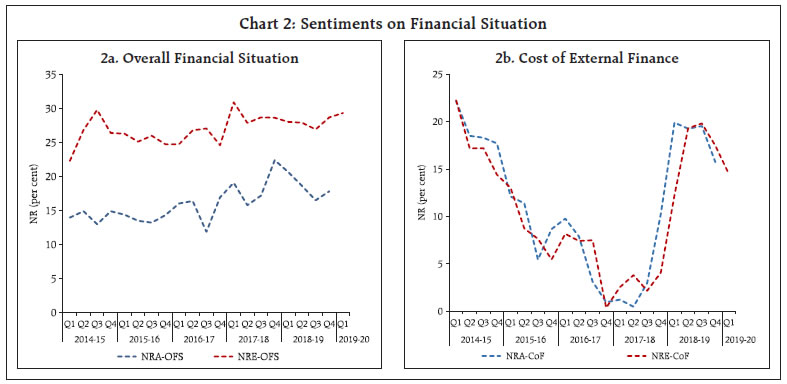
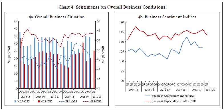
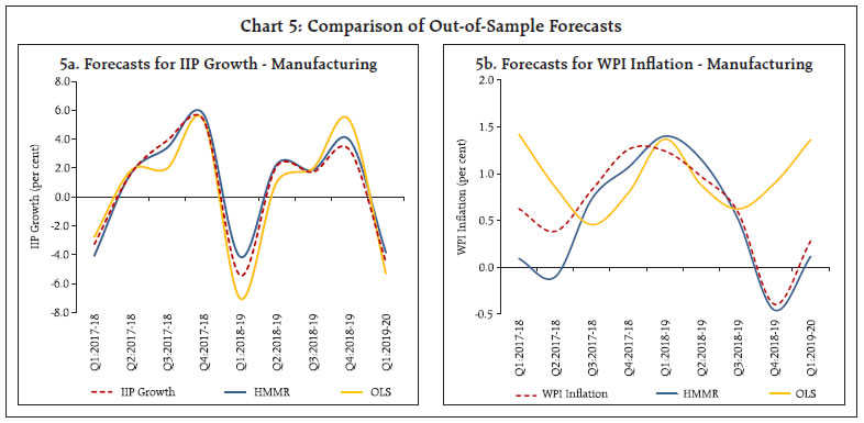
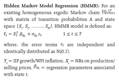
Early indicators from the Industrial Outlook Survey – an indispensable tool of policy makers to gauge economic condition – point to steady demand conditions during 2018-19, with optimism moderating in the first quarter of 2019-20. As an outcome of concerted efforts towards boosting demand, survey responses suggest improvement in financing conditions in Q1:2019-20. On the prices front, the softening in input costs, especially of raw materials, are being passed on to consumers leading to softening of selling prices. Forecasts based on Hidden Markov Model (HMM) regression using responses from the survey were found to track the movements of the index of industrial production (IIP) growth and wholesale price index (WPI) inflation for the manufacturing sector.

Introduction

In the array of instruments used by policy makers to gauge current economic environment and to help in short-term forecasts, business outlook surveys assume the prime spot. These surveys yield crucial—albeit qualitative—information, with added advantage of being low cost and easily accessible tools in forecasting turning points in the business cycle (OECD, 2003). These surveys have been profoundly used to get an “informed opinion” about economic trends in key industries in a forward-looking manner (Vincent 2006). With the inception of its quarterly Industrial Outlook Survey (IOS) in 1998, the Reserve Bank emerged as a forerunner among emerging market economies (EMEs) in conducting such surveys.

Against this backdrop, the aim of the article is two-fold: first, with a benefit of hindsight, the article presents the key messages emanating from the survey and analyses how closely the survey indictors track related macroeconomic aggregates primarily the IIP and WPI during 2018-19. Second, taking a longer time horizon from Q1:2000-01 to Q1:2019-20, and employing novel econometric technique of Hidden Markov Model Regression (HMMR), the usefulness of IOS in tracking the turning points in business cycles is established.

The rest of the article is organised into five sections. Section 2 summarises cross-country experience in business tendency surveys and provides a brief literature review on HMMR in analysing survey inputs. Section 3 presents an overview of the stylised facts on select parameters of manufacturing conditions that were surveyed during 2018-19. Section 4 provides evidence that the indicators of IOS forecast business cycle turning points accurately. Section 5 concludes the findings of the article.

2. Literature Review

Business tendency or outlook surveys have a history dating back to as early as 1920s and they have been implemented by an increasing number of countries over the years. Some of the earliest surveys were conducted by trade associations such as, the Confederation of British Industries and the Ifo Institute for Economic Research in Germany. Central banks in countries like Japan and Belgium have been carrying out such surveys to gauge advance information on economic situation before the release of official data. Among member countries of the Organisation for Economic Cooperation and Development (OECD), Canada, Australia, transition countries in Europe and Central Asia sponsor a handful of business tendency surveys which are being conducted by their national statistical offices, private or public. Some of the most prominent business outlook surveys are conducted and released by private institutes such as the Conference Board and Thompson Reuters in the United States.

As part of its joint harmonised European Union (EU) programme of surveys, the Directorate General for Economic and Financial Affairs (DG ECFIN) of the European Commission addresses regular surveys to the industry representatives of the EU and candidate countries. In this league, Centre for International Research on Economic Tendency Surveys (CIRET)– a forum for leading economists and institutions that conduct and analyse surveys can be credited for much of the early developments as well as recent improvements in business tendency surveys.

Business Tendency/Outlook Surveys gather information about a wide range of variables including production, order books, stocks of finished goods, employment and prices. Literature suggests that since such series do not undergo drastic revisions, they are useful in predicting turning points in the business cycle (OECD, 2003). As the survey responses help in monitoring and forecasting business cycles, they are used widely by a broad spectre of economic agents. The data series are usually seasonally adjusted and the cyclical profiles are easy to detect given the absence of long-term trend in such responses.

Before employing the indicators gathered through such surveys, it is important to establish that such information truly tracks the business cycles. The Markov-switching (MS) regression or hidden Markov models (HMM)¹ for regression techniques have an edge over other techniques such as ordinary least square (OLS) because of ability to capture asymmetry in business cycle expansion and recession (Burns and Mitchell, 1946).

Extensions of HMMs to determine the growth rates and business cycle turning points were studied by Hamilton (1989). Later, Diebold and Rudebusch (1996), Kim and Nelson (1998), Filardo and Gordon (1999), Chauvet (1998) and Camacho et al. (2012) combined the characteristics of factor models and MS models by allowing MS features in determination of factor. Such time-varying MS regression models have found applications in capturing business cycle fluctuations from leading indicators for the French economy (Bardaji, 2009), studying the economic situation in Poland (Bernardelli, 2015), detecting turning points in the American business cycle (Bellone and Saint-Martin, 2003).

In the Indian context, previous research has already shown that factor indices derived from responses to IOS yield lead indicators for tracking manufacturing activities in India (Ansari and Majumdar, 2019). The present work aims to supplement the existing research in this area by exploring the application of MS regression models using survey responses for detecting turning points in the Indian business cycle.

3. IOS in 2018-19: Some Stylised Facts

The Reserve Bank’s IOS encompasses a panel of 2,500 manufacturing companies with paid-up capital of above ₹ 50 lakhs, which undergoes periodic revision with addition of newly formed companies and removal of closed or merged companies. The respondents comprise of senior management personnel or finance heads of enterprises and the response rate hovers around 45-50 per cent. The survey schedule seeks responses to qualitative questions on 23 parameters² to gauge information about the current situation as well as outlook/expectations for the next quarter. The questions on stock variables (viz., production capacity, pending orders, level of capacity utilisation, inventories) seek a comparison with the normal situation, whereas, sequential responses, i.e., changes over the previous quarter, are sought for flow variables (viz., change in production, order books, exports, imports, availability of finance).

3.1 Methodology

The survey responses are quantified using single summary statistic called the Net Response (NR), which is generally defined as the difference between the proportions of optimistic and pessimistic responses. NR can take values spanning from -100 to +100. Positive values of NR signal growth/ optimism while a value below zero indicates contraction/ pessimism³. The zero value is interpreted as ‘status quo’. However, for sake of comparison with the target macroeconomic indicators in this article, we have maintained the convention of defining NRs of all parameters as the excess of proportion of respondents indicating “increase” from that indicating ‘decrease’, thus positive NR would indicate an ‘increase’ and negative value of NR would signify a ‘decline’. In the rest of this article, the proportion of respondents indicating “no change (NC)”, has also been included in conjunction with the NRs for comprehensive presentation.⁴

3.2 Demand Conditions

Sentiments of Indian manufacturers on select parameters such as production (PR), order books (OB), capacity utilisation (CU), stock of raw material inventories (INV) and employment (EMP) are indicative of aggregate demand conditions in the economy.

The net responses for assessment of production (NRA-PR) during 2018-19 maintained proximity with the peak level of recent years which was attained in Q4:2017-18, pointing to steady demand conditions during the period. During the year, net responses on expectations of production (NRE-PR) perceived a quarter back was found to co-move with the assessment realised subsequently⁵. Expectations for Q1:2019-20 pointed to some moderation as compared to Q4:2018-19. Feedbacks of manufacturers on production, as captured by NRA-PR and NRE-PR, broadly corroborate the trend traced out by the quarterly growth of IIP (Chart 1a). The proportion of respondents indicating “no change” on production (NCA-PR and NCE-PR) hovered around 48 per cent during the entire period.

Manufacturers’ perceptions on another indicator of demand such as order books (OB) mirrored their views on production largely in both assessment and expectations periods. While order books dipped slightly in Q3:2018-19 and thereafter remained stable in Q4:2018-19, the outlook for Q1:2019-20 showed some moderation from Q4 (Chart 1b). Capacity utilisation outlines the portion of installed capacity actually utilised by an enterprise in its production process and is recorded by a quantitative survey of the Reserve Bank, namely order books, inventories and capacity utilisation survey (OBICUS) for the Indian manufacturing sector. The assessment on CU, as captured by the IOS, evolved in the direction similar to the actual CU as measured by OBICUS and the outlook for the first quarter of 2019-20 was seen to moderate in concordance with the movement of actual CU (Chart 1c).

Employment, another yardstick to gauge business climate, is captured in the survey and the parameter includes all cadres of employees (like part-time, full-time and casual labourers). Sentiments on employment had been on an improving spree for four consecutive quarters till Q1:2018-19, which was followed by a dip in Q2:2018-19 and remained stable through the remaining part of the year. The proportion of responses indicating “no change”, typically around 75 per cent, tends to dominate the responses on this parameter (Chart 1d).

Inventories of raw materials (IRM) witnessed gradual ascent starting Q1:2017-18 which sustained in the outlook for Q1:2019-20. The responses to this parameter can be mainly categorised as NC (at around 80 per cent) since companies generally set a fixed level of raw materials except during periods of large variations in demand and/or prices (Chart 1e).

3.3 Financial Situation

A sound financial situation of a company is reflective of its own strength as well as overall optimistic business environment, giving an impetus to investments. During 2018-19, the respondents expressed waning optimism on overall financial situation (OFS) for the first three quarters, with slight improvement in the fourth quarter which sustained in the outlook for Q1:2019-20 (Chart 2a). Manufacturers indicated edging up of cost of external finance (CoF), as reflected by the gradual shoring up of NRs from the onset of 2018-19; however, Q1:2019-20 pointed to some respite (Chart 2b).

3.4 Price Scenario and Profitability

Net responses on select parameters such as cost of raw materials, selling prices and salary outgo relay the sentiments on price scenario in the manufacturing sector. Cost of raw materials (CRM) spiked up during the initial half of 2018-19 and eased thereafter. The survey feedbacks on CRM closely track the movements in WPI inflation for raw materials (Chart 3a).

Mellowed input costs, especially of raw materials, were passed on to consumers leading to softening of selling prices to some extent, as indicated by descending NRs on selling prices (SP) from Q2:2018-19 (Chart 3b).

The interplay between input costs incurred during production process and selling prices (ex-factory unit prices) bear significance in determining the profit margin of manufacturers. Recovery in profit margins (PM) (gross profits as percentage of net sales) from Q3:2018-19 mostly stemmed from alleviated cost pressures. Expectations on profit margins for Q1:2019-20 continued to be positive (Chart 3c).

3.5 Overall Business Conditions

Manufacturers also expressed their views about the business ambience, in general. Nearly half of the respondents polled that the overall business conditions were slated to maintain “status quo” through 2018-19. NRs based on the opinion of the rest of the respondents remained positive through the reference period, though there was a marked cautious descent from its level in Q4:2017-18. The outlook for Q1:2019-20 remained steady at a level since Q3:2017-18 (Chart 4a).

The NRs on select business parameters are combined into composite indices⁶ namely, business assessment index (BAI) and business expectations index (BEI) to portray the prognosis of business climate in a snapshot. By construction, the index ranges from 0 to 200 with the 100 mark separating expansion from contraction. The index declined slightly from its level in Q4:2017-18, however, remained in the zone of expansion throughout 2018-19. BEI for Q1:2019-20 stood at 113.5, sliding down from 116.2 in Q4:2018-19 (Chart 4b).

4. Empirical Analysis: An Alternative Approach to Study Dynamics of Manufacturing Activity

In order to evaluate how well the net response (NR) indicators track business cycle, the Hidden Markov Model Regression (HMMR) technique was employed in line with the existing literature (Bardaji, 2009; Bernardelli, 2015; Bellone and Saint-Martin, 2003). With an aim to develop a robust relationship between survey parameters and related macroeconomic indicators, data spanning from Q1:2000-01 to Q1:2019-20 was considered for the purpose of analysis. The entire sample of observations was bifurcated into training and test sets after seasonal adjustment. For exploration purpose, a simple two-regime Markov model was considered. Macroeconomic indicators for manufacturing demand and prices viz., manufacturing IIP growth and manufacturing WPI inflation, were regressed on NRs (expectations) on production and selling prices respectively, to obtain estimates of regression parameters for each state of the underlying Markov process (Annex - I). Out-of-sample predictions corresponding to Q1:2017-18 till Q1:2019-20 for the dependent variables and states of the underlying unobserved Markov chain were made on a rolling basis and an additional data point was incorporated at each successive iteration⁷.

For comparison purpose, ordinary least squares (OLS) regression was performed on the same set of time series observations and out-of-sample forecasts were calculated likewise on a rolling window. The findings suggest that the HMMR model forecasts both macro indicators of demand and prices better as compared to OLS regression model (Table 2). While forecasts based on both HMMR and OLS were found to move in tandem with actual manufacturing IIP growth, HMMR tracked IIP more closely in comparison (Chart 5a). Trajectory of manufacturing WPI inflation, on the other hand, was portended with more accuracy by forecasts based on HMMR (Chart 5b).

5. Concluding Observations

The four rounds of IOS conducted during the year 2018-19 indicated optimistic demand conditions as evident in sentiments on production, order books, capacity utilisation and employment; though, the outlook for the first quarter of 2019-20 remained subdued. The overall financial situation, though garnered optimism from majority of respondents, waned off gradually during the year with Q1:2019-20 pointing to some improvement. Manufacturers allayed concerns regarding cost of external finance. On the prices front, sentiments on input costs showed softening of pressures on enterprises, especially during the latter half of 2018-19, which translated to reduced burden on consumers in terms of lower selling prices. Forecasts based on HMMR model using responses from the survey were found to track the movements of IIP growth and WPI inflation for the manufacturing sector.

References

Amstad, M. and Richard, E. (2000). “A New Approach to indicate Changes in Business Cycles in the Manufacturing Industries Using Markov Switching Models on Business Survey Indicators in Economic Surveys and Data Analysis”, CIRET Conference Proceedings, pp. 283-305.

Ansari, J. and Majumdar, S. (2019). “Business Sentiments and Expectations in 2017-18”, RBI Bulletin, January.

Artis, M. J., Marcellino, M. and Proietti, T. (2004). “Dating Business Cycles: A Methodological Contribution with an Application to the Euro Area”, Oxford Bulletin of Economics and Statistics 66, 537–565.

Bardaji, J., Clavel, L. and Tallet, F. (2009). “Constructing a Markov-switching Turning Point Index Using Mixed Frequencies with an Application to French Business Survey Data”, Journal of Business Cycle Measurement and Analysis, vol. 2009/2, 111-132.

Bardaji, J. and Tallet, F. (2009). “Detecting Economic Regimes in France: A Turning Point Index using Mixed Frequency Data”, INSEE (France).

Baum, L.E., Petrie, T., Soules, G. and Weiss, N. (1970). “A Maximization Techinque occurring in the Statistical Analysis of Probabilistic Functions of Markov Chains”, Annals of Mathematical Statistics, 41,164–171.

Bellone, B. and Saint-Martin, D. (2003). “Detecting Turning Points with Many Predictors through Hidden Markov Models”, French Forecasting and Economic Analysis Directorate.

Dua, P. and Roy, B. (1997). “Consumer Confidence and the Probability of Recession: A Markov Switching Model”, Working Papers 47, Centre for Development Economics.

Duprey, T. and Klaus, B. (2017). “How to predict financial stress? An assessment of Markov switching models”, Working Papers 2057, European Central Bank.

Eurostat in collaboration with the Conference Board, (2017). ‘Handbook of Cyclical Composite Indicators’.

Gregoir, S. and Lenglart, F. (2000). “Measuring the Probability of a Business Cycle Turning Point by Using a Multivariate Qualitative Hidden Markov Model”, Journal of Forecasting, 19, 81-102.

Hamilton, J.D. (1989). ‘A new approach to the economic analysis of non-stationary time series and the business cycle’, Econometrica, 57, 357-384.

Hansson, J., Jansson, P. and Lof, M. (2003), “Business Survey Data: Do They Help in Forecasting the Macro Economy?”, Working Papers 84, National Institute of Economic Research.

Kabundi, A. (2006). “Estimation of Economic Growth in France Using Business Survey Data”, Working Papers 04/69, IMF.

Kim, CJ. And Murray, CJ .(2002). “Permanent and Transitory Components of Recession”, Empir Econ, 27,163-183.

Morier, B. and Teles, V. (2016). “A Time-Varying Markov-Switching Model for Economic Growth”, Macroeconomic Dynamics, 20, 1550-1580.

OECD, (2003). “Business Tendency Surveys: A Handbook”.

United Nations, (2015). “Handbook on Economic Tendency Surveys”.

Zucchini, W. (2005). “Hidden Markov Models for Time Series: An Introduction Using R”, 2nd ed., 370 pp., Boca Raton, FL: CRC Press, Taylor & Francis Group.

Annex - I

The parameter estimates in the training sample are presented in Table A1 and A2 for regressions on IIP growth and WPI inflation respectively.

Fundamental assumption of the model is that at any time point, the time dependencies between the observations are due to time-dependencies between the states assumed to follow a first-order Markov process. For hidden Markov models, the marginal log-likelihood of the observations is computed by forward-backward algorithm (Baum et al.1970) and the parameters are estimated by iteratively maximizing the expected log-likelihood.

State Estimation: The Viterbi-algorithm (Zucchini 2005) globally decodes the underlying hidden Markov state and predicts the most probable sequence of Markov states given the observed dataset. This is done by determining the sequence of states (s₁, s₂, …. , s_N) which maximises the joint distribution of the hidden states given the entire observation process, i.e., argmax Pr(S₁= s₁, S₂= s₂,… S_N= s_N|y₁,…., y_t, x₁,…, x_t) For expositional purposes, we have attempted two states, though there is some empirical evidence that three states, representing recession, high growth and normal growth, can lead to improvements (Kim and Murray 2002 for US economy, Artis et al. 2004 for the Euro area).

Initial state probabilities assumed State 1 as certain, i.e., probability=1. The transition matrix is given as:

Initial state probabilities assumed State 1 as certain, i.e., probability=1. The transition matrix is given as:

^* This article is prepared by Sayantika Bhowmick and S. Majumdar, Division of Enterprise Surveys, Department of Statistics and Information Management (DSIM). The views expressed in the article are those of the authors only. The latest round of the survey data was released on February 6, 2020 on the RBI’s website at /en/web/rbi/-/publications/industrial-outlook-survey-of-the-manufacturing-sector-for-q3-2019-20-revised-lt-span-gt-19415. The previous article was published in January 2019 issue of the RBI Bulletin and can be accessed at /en/web/rbi/-/publications/rbi-bulletin/business-sentiments-and-expectations-in-2017-18-17996.

¹ For an existing unobserved or hidden Markov chain on state space S, an observed time series is related to a set of covariates through different regression planes. The regression planes depict the relationship between the dependent and independent variables with distinct regression parameters under different states of the unobserved Markov chain (Annex - I).

² Parameters are overall business situation, financial situation, working capital finance requirement, availability of finance, production, order books, cost of raw material, cost of finance, inventory levels (both raw material and finished goods), employment, exports, imports, capacity utilisation indicators, selling prices and profit margins.

³ Usually, an increase in NR is considered to be optimistic in case of demand parameters such as production, order books, capacity utilisation etc., price indicators like selling prices. Though, for all cost related parameters such as cost of raw materials, cost of finance etc., a decrease in NR signifies optimism. However, this convention has not been used in this article.

⁴ If I, N and D represent the percentage of increase, no change and decrease to a particular parameter then NR = 100 × (I – D) and NC = 100 × N. For example, if the proportions of respondents indicating an “increase”, “no change” and “decrease” in the study variable as compared to the previous quarter are 15 per cent, 85 per cent and 0 per cent respectively, net response of 15 per cent would reveal that respondents assessed an “increase” in the study variable, overshadowing the fact that a majority proportion voted for “no change” in consensus. On the other hand, if the respective proportions are 48 per cent, 4 per cent and 48 per cent, net response of 0 per cent in this case might lead to conclude about a no-change scenario, whereas, in reality such situation depicts a case of complete disagreement among the respondents resulting in inconclusive direction of movement of the target variable. In general, NC of at least 50 per cent would lead to more conclusive consensus of “status quo” among respondents. Therefore, very high or low values NCs are presented in charts.

⁵ NRA-PR and NRE-PR denote the net responses for assessment and expectation on production. NCA-PR and NCE-PR are proportions of no-change responses for assessment and expectations on production. These representations are uniformly used for all other parameters discussed in this article. Likewise, the corresponding measures have been used for other parameters such as order books (OB), employment (EMP), inventory of raw materials (IRM), capacity utilisation (CU), overall financial situation (OFS), cost of external finance (CoF), cost of raw materials (CRM), selling prices (SP), profit margins (PM) and overall business situation (OBS).

⁶ The Business Assessment and Expectations Indices are composite indicators derived as weighted average (share of GVA of different industry group) of net response on (1) overall business situation; (2) production; (3) order books; (4) inventory of raw material; (5) inventory of finished goods; (6) profit margins; (7) employment; (8) exports; and (9) capacity utilisation.

⁷ Forecasts were re-adjusted with corresponding seasonal factors for ease of comparison with the target macro-economic indicators.

⁸ OLS regression models were evaluated on one-quarter, two-quarters, three-quarters and four-quarters growth of respective macro-economic variables. Based on lowest error measures of in-sample predictions, one-quarter growth of macro indicators of demand and price were regressed on the corresponding NRs from survey for the purpose of the study.