 IST,
IST,


Measuring Productivity at the Industry Level - The India KLEMS Database
|
This document describes the procedures, methodologies and approaches used in the construction of India KLEMS database version 2024. The dataset includes measures of Gross Value Added (GVA), Gross Value of Output (GVO), Labour Employment (L), Labour Quality (LQ), Capital Stock (K), Capital Composition (KQ), the consumptions of Energy (E), Material (M) and Services (S) inputs, Labour Productivity (LP) and Total Factor Productivity (TFP). The database covers 27 industries comprising of the entire Indian economy. The database also provides these estimates at the broad sectoral levels (agriculture, manufacturing and services) and at the all-India levels. In the current version of the database covers the period from 1980-81 to 2022-23. The series have been constructed on the basis of data compiled from NSO, NSSO, ASI, Input-Output tables (I-O tables) and processed according to appropriate procedures. These procedures were developed to ensure harmonization of the basic data, and to generate growth accounts in a consistent and uniform way. Harmonization of the basic data has focused on several areas such as industrial classification, and aggregation levels. The production and publication of India KLEMS database are meant to support empirical research in the area of economic growth and its sources. Most importantly, the database is meant to support the conduct of policies aimed at supporting the acceleration of productivity growth in the Indian economy. The India KLEMS database, in this regard, provides a comprehensive measurement tool to monitor and evaluate productivity growth in the Indian economy. Finally, the construction of the database would also support the systematic production of reliable statistics on growth and productivity using internationally comparable methodologies based on India’s national accounts, input-output tables and labour market surveys. The work relating to compilation of India KLEMS data was being done by the India KLEMS team housed at the Centre for Development Economics, Delhi School of Economics until the end of 2020. The work has been shifted to the KLEMS Division of the Department of Economics and Policy Research of RBI since February 2021The current version of the India KLEMS Database, released hereby, is the third independent compilation of this data by the KLEMS Division in RBI, after the previous release of the data in January 2024. 1.2 Coverage: Industries and Variables In this section we describe the coverage of India KLEMS database in terms of industries and variables. The database is created for 27 industries. The industrial classification is constructed by building concordance between NIC 2008, NIC 2004, NIC 1998, NIC 1987 and NIC 1970 to generate a uniform definition of ‘industries’ since 1980-81. This classification is very close to the International Standard Industrial Classification (ISIC) revision 3. The 27 industries are aggregated to form six broad sectors, namely:
Table 1.1 provides a list of the 27 industries, including the higher aggregates. For detailed classification and concordance of study industries with NICs, readers may refer to Version 8 of the manual published in 2022. Table 1.2 provides an overview of all the series included in our database. Measures of Capital (K), Labour (L), Energy (E), Material (M) and Service (S) inputs as well as Gross Output (GO), have been constructed using National Accounts Statistics (NAS), Annual Survey of Industries (ASI), NSSO rounds and Input-Output (IO) Tables. In building annual time series on gross output, five inputs and factor income shares, various assumptions are made to fill up gaps in industry details and link series over time. As we know that NSSO rounds of unregistered manufacturing, Input Output Transaction Tables, and Employment and Unemployment Surveys by NSSO are available only for certain benchmark years, the use of information from these data sources necessitates interpolation and assumption of constant shares for building a series of output and inputs. However, as the successor of NSSO's Employment Unemployment Survey, the Periodic Labour Force Survey (PLFS) data has become available annually since 2017-18, the labour input series no longer requires any extrapolation. The labour input series is being updated under each round of India KLEMS using available survey data from PLFS only. Chapter 2: Gross Value-Added Series at the Industry Level This chapter describes the data sources and methodology used to construct the Gross Value Added (GVA) series at current and constant prices for 27 study industries for the period of 1980-81 (1980) to 2022-23(2023). The National Accounts Statistics (NAS) brought out by the NSO (National Statistics Office, Government of India) is the basic source of data for the construction of series on gross value added for INDIA KLEMS-industries. Up to 2011-12, estimates of GVA at both current and constant (2011-12) prices for all industries are obtained from Back Series of National Accounts (Base 2011-12). For years after 2011-12, they are directly obtained from NAS 2023. However, NAS estimates of value added are not available for a few India KLEMS industry groups. Therefore, we had to split some of the aggregate industry groups from NAS. Maintaining consistency with NAS, the value-added data in India KLEMS is measured at basic price. The construction of Gross valued added series involves three steps. Step 1: A concordance table between the classification used in the NAS and the 27 study industry classification used for this project has been prepared. Further, concordance between all the 27 sectors has been constructed with NIC- 1970, 1987, 1998, 2004 and 2008. Out of the 27 study industries, for 20 industries, GVA series both in current and constant prices is directly taken from NAS1. The sectors for which data are provided in NAS are Agriculture, Forestry & logging, Fishing, Mining and Quarrying, Manufacturing, Electricity, gas and water supply, Construction, Trade, Hotels & Restaurants, Railways, Transport by other means, Storage, Communication, Banking & insurance, Real estate, Ownership of Dwelling & Business Services, Public Administration & Defense and Other Services. Step 2: For manufacturing industries where direct estimates of GVA were not available from NAS, estimates have been made using additional information from ASI and NSSO unorganised manufacturing data. In these cases, GVA data is constructed by splitting the NAS data using ASI or NSSO distributions. ASI data (annual) has been used for registered and corporate manufacturing, whereas interpolated ratios from NSSO 40th (1984-85), 45th (1989-90), 51st (1994-95), 56th (2000-01), 62nd (2005-06), 67th round (2010-11) and 73rd round (2015-16) rounds have been used for Unregistered and household manufacturing segments. For unregistered manufacturing for years 2015-16 to 2022-23 the ratio obtained from 73rd round of unregistered manufacturing has been used for the splitting. Table 2.1 and Table 2.2 showcase the methodology used to split GVA of certain NAS sectors to match concordance with our classification. It is important to note that the industry-level value-added volume indices are based on NAS. NSO provides single-deflated value-added estimates for all sectors except Agriculture. Step 3: According to India KLEMS, GVA is adjusted for Financial Intermediation Services Indirectly Measured (FISIM). The detailed method of FISM adjustment is provided in earlier versions of the KLEMS manual. Chapter 3: Gross Output Series at the Industry Level This chapter describes the procedures and methodologies used in constructing the database for gross output series at the industry level over the period 1980-81(1980) to 2022-2023(2023). To construct the gross output series at industry level, we use multiple data sources namely National Accounts Statistics, Annual Survey of Industries, NSSO rounds for unorganized manufacturing and Input Output Transaction tables. The data sources and methodology used are documented below: National Accounts Statistics: The NAS is the basic source of data for the construction of time series on the gross output. For years since 2011, we have taken the estimates of GVO both at current and constant prices for all industries directly from NAS 2024. (a) Filling procedures of National Accounts series: It is to be noted that the NAS estimates of gross output for a few industry groups are at a more aggregate level, requiring splitting of the aggregates. In such cases, NAS estimates of output have been split using additional information from the Annual Survey of Industries and NSSO rounds of Unregistered Manufacturing to obtain estimates at a higher level of disaggregation. Secondly, for Unregistered manufacturing, gross output data is available in NAS from 2004-05 onwards. In this case, information from NSSO survey rounds has been used for missing years to derive output estimates of unregistered manufacturing industries at current and constant prices. As mentioned earlier, for the gross value-added series of service sectors, we obtain our estimates from NAS. However, prior to 2011-12, National Accounts did not provide any estimates of the gross output of service sectors and hence we rely on Input output transaction tables (from which the ratio of gross to value added is computed which is then applied to GVA reported in NAS) which are available at an interval of 5 years or so. This necessitates interpolation and assumption of constant shares for measuring output of services sectors. The Input Output Transaction Tables for Benchmark years of 1978-79, 1983-84, 1989-90, 1993-94, 1998-99, 2003-04 and 2007-08 are used to derive gross output series for service sectors. The construction of the gross output series at current and constant prices involves the following steps: Step 1: Measuring Gross Output of Agricultural Sector, Mining and Quarrying, and Construction NAS provides nominal and real GVO series for a) Crops and Plantation, b) Animal Husbandry c) Forestry and Logging d) Fishing. By aggregating the GVO of these four subsectors we derive the GVO of Agricultural sector. The Gross output estimates of Mining and Quarrying and Construction at current and constant prices from 1980-2023 is also directly taken from NAS. Step 2: Measuring Gross Output of Manufacturing Industries Since 2011-12, gross output data for 7 out of 13 manufacturing industries listed in table 3.1 are directly picked up from NAS. For the remaining 6 sectors output is constructed by splitting the NAS output data using ASI or NSSO distributions. ASI data (annual) has been used for registered manufacturing whereas interpolated ratios from 67th (2010-11) and 73rd (2015-16) rounds have been used for Unregistered Manufacturing segments. A list of study industries is presented in Table 3.2 showcasing the methodology used to split GVO of certain NAS sectors to match concordance with our classification for the year 2011 to 2023. Step 3: Measuring Gross Output for Services Sectors and Electricity, Gas and water supply Since 2011 -12 NAS provided estimates of GVO at current and constant prices. Prior to 2011-12 Gross Output series for Services sectors and sector Electricity, Gas and Water supply have been constructed using information from Input – Output Transaction Tables of the Indian economy published by CSO. The details method of construction of GVO back series for services is provided in earlier versions of KLEMS Data manual. Chapter 4: Labour Input Series at the Industry Level This chapter discusses the construction of labour input for 27 industries from 1980-81 to 2022-23. Labour input captures both the quantity of labour (i.e. number of persons) and quality of labour over time. Labour quality is measured based on educational qualification and wage rates of the workers within each of the 27 industries. Given the limitations of India’s employment statistics (Sivasubramonian; 2004, & Himanshu; 2011, Ghose; 2016), especially the availability of information on wages/ earnings of different category of workers across industries, the database provides only the labour quality index based on five different education categories. Labour input is measured by multiplying the number of persons employed by the index of labour quality which captures the human capital embodied in the labour, constructed separately for each industry. The 38th to 68th rounds of the Employment and Unemployment Survey (EUS) by India’s National Sample Survey Office (NSSO) conducted between 1983 and 2011-12, respectively, and all the annual Periodic Labour Force Survey (PLFS) rounds from 2017-18 to 2022-23 by National Statistical Organization (NSO) are the main sources data for estimating labour input. We use India’s decadal census and population projections based on Government of India’s various reports for estimating India’s population. Methodology The total employment, measured by the number of persons engaged in each of the 27 industries in India is computed as follows:
For extrapolation backward to 1980-81 to 1982-83, the interpolation of the broad industrial classifications of 32nd round (1977-78) and 38th round (1983-84) are used. Thus, the estimates from 32nd round are mainly used as control numbers. Between 2005 and 2011, we observed very high growth rate in number of employed persons series for the industry Electrical and Optical Equipment as compared to other manufacturing industries and the overall growth in employment in this industry during 2005-2011 was found to be higher than that for Construction (which seems somewhat unrealistic). It was also observed that there was a negative growth in employment in Textiles, Textile Products, Leather and Footwear although real GVA of this industry more than doubled between 2005 and 2011. To address these issues, some adjustments to the initial employment estimates for Electrical & Optical Equipment and Textiles, Textile Products, Leather and Footwear have been done.Onwards 2005, employment series for Electrical & Optical Equipment has been estimated applying annual growth rates obtained from ASI and NSSO rounds to the number of employed persons for the year 2005-06. Then, for the years 2005-06 to 2011-12, we compute the difference between estimated employment series from EUS rounds and that based on ASI & NSSO rounds for the Electrical and Optical Equipment industryand add it to Textiles, Textile Products, Leather and Footwear industry. This ensures that for the manufacturing as a whole our estimates remain the same as obtained from EUS rounds. 4.2 Estimation of Labour Quality index The quality of labour force is of considerable importance in the context of productivity measurement, and one of the widely used methodologies to capture changes in labour quality is given by Jorgenson, Gollop and Fraumeni (JGF) (1987). In growth accounting methodology of measurement of total factor productivity (TFP) when output growth is decomposed into growth of inputs and the residual TFP, then labour input is measured as an index of labour service flows. It accounts for changes in labour quality in terms of labour characteristics such as educational attainment, age (experience), gender, employment status, etc. and thus accounts for heterogeneity of the labour force. In our study, the index of aggregate labour quality measures the changes in the composition of labour in the economy. The present study has computed labour quality index by using only education characteristic in the JGF methodology. Thus, the data required for the labour quality index in the present case, is employment and earnings by education and by industry. The labour quality index has been computed using five education categories namely- up to primary, primary, middle, secondary & higher secondary, and above higher secondary. There are thus five types of persons employed for each of the 27 study industries. The quality growth rates are estimated for total persons employed in these industries in India for the 38th, 50th, 55th, 61st, 68th rounds of EUS by NSSO, and all the PLFS rounds since 2017-18. They are then indexed to 1983-84 (38th round) as the base, so as to assess the temporal changes in labour’s skill. Interpolation has been done between the major rounds for values of the intermediate years. Since the series is required from 1980-81, we have extrapolated it backwards from 1983-84 and the index is recomputed with base 1980-81 equal to 100. The following steps have been performed:
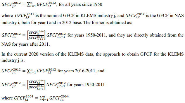
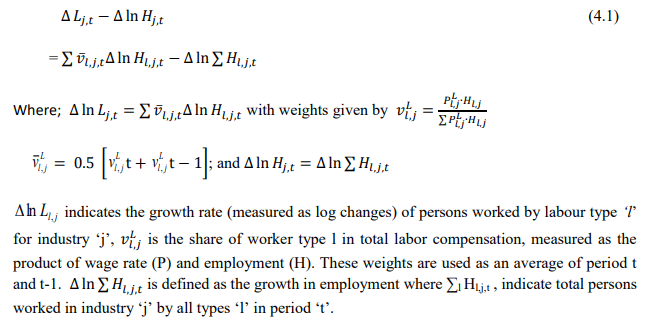 The first term of equation 4.1 indicates the changes in labour quality index, which is due to the changes in the composition of workers and the second term indicates the change in total persons employed in sector ‘j’. The index of aggregate labour quality thus measures the changes in the composition of labour in the economy The labour input (adjusted labour persons) then can be obtained by multiplying the number of persons employed by the corresponding labour quality index and the labour input growth is finally obtained by combining the growth of persons employed and the growth in the index of labour quality. Chapter 5: Capital Services Series at the Industry Level This chapter outlines the methodology employed to estimate capital Services for the 27 industries in India KLEMS database version 2024. All the productivity calculations in India KLEMS use capital services as an input to production, which is estimated using the approach developed by Jorgenson and Griliches (1967), and outlined in Jorgenson, Gollop, and Fraumeni (1987). The estimation of capital service growth rate is accomplished by first estimating capital stock for different assets, and then aggregating them across assets after correcting for the differences in their marginal productivities. Capital services account for the differences in marginal productivity between different asset types while capital stock measures only the vintages of capital, they do not account for asset heterogeneity. For instance, aggregate capital stock measures would assume that a computer's productivity is the same as that of a car. However, proper measures of capital stock would account for the decline in the efficiency of both computers and cars over their lifetime. Following an overview of the theoretical method to measure capital services (Jorgenson and Griliches,1967; JGF, 1987), the chapter discusses the specific empirical approaches we follow to implement these methods within the constraints of data availability for Indian industries. In India KLEMS, we have reported capital stock, capital services and the capital “capital composition effect”. Capital stock is reported in constant price volumes, and growth rates, while the latter two are reported in growth rates and indices. To measure capital services, using the Jorgenson and Griliches (1967) approach, we need estimates of capital stock for detailed asset types and the shares of each of these assets in total capital remuneration. The aggregate capital services growth rate is derived as a weighted growth rate of individual capital assets, the weights being the shares of each asset in the total compensation made to capital, i.e, 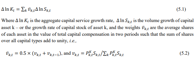 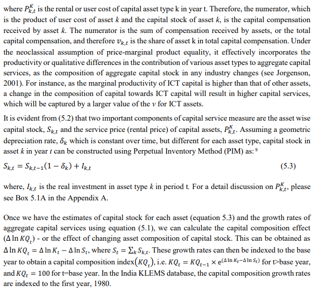 Since our measure of capital input takes account of asset heterogeneity, it was essential to obtain investment data by asset type. We distinguish between 3 different asset types – construction, transport equipment, and machinery (includes ICT and non-ICT machinery).10 We exploit multiple sources of information for the construction of our database on capital services. This includes the National Accounts Statistics (NAS) that provide information on broad sectors of the economy, the Annual Survey of Industries (ASI) covering the organized manufacturing sector, the National Sample Survey Office (NSSO) rounds for unorganized manufacturing and various Input-Output tables. Even though we use multiple sources of data, our final estimates are fully consistent with the aggregate data obtained from the NAS. In addition, our approach to capital measurement is consistent with international practices such as the EU KLEMS11, which ensures the possibility of international comparisons. In what follows, we discuss the various sources of data for asset wise investment and the construction of the relevant variables, in detail. (a) Asset-wise investment for broad sectors of the economy Industry-level estimates of capital input require detailed asset-by-industry investment matrices. NAS provides information on aggregate capital formation by industry of use for nine broad sectors, which, nevertheless, was not sufficient for our purpose. Therefore, we have collected more detailed data on assets and industries from the CSO12. This is the data underlying the published aggregate gross fixed capital formation by the broad industry groups, separately for public and private sectors. For those sectors for which the investment matrices were not available from CSO, we gather information from other sources (e.g. ASI for organized manufacturing and NSSO surveys for unorganized manufacturing) and benchmark it to the aggregate investment series from the National Accounts. The data used in the current version of the India KLEMS is based on the revised NAS with 2011-2012 base and is available only since 2012. Therefore, for earlier years, we extrapolate the series using growth rates from previous version of the data. Table 5.1 provides an overview of asset types available in NAS and their corresponding asset types used in our study. Investment in education and health are obtained directly from national accounts for the period after 2012, for each asset. For years before 2012, we assume the trend in the distribution of output, in order to split the total investment in the aggregates of these sectors into sub-sectors.
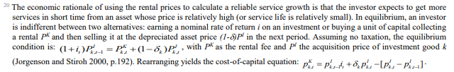
Total investment in each asset category is calculated as the sum of private and public-sector investment in each asset. Investment in transport equipment was not available separately for the private sector industries. Therefore, we distributed the NAS total machinery in the private sector using the industry distribution of machinery and transport equipment. These estimates are then subtracted from each industry’s total machinery & transport equipment data to obtain the transport equipment investment in the private sector industries. Using this approach, we could generate investment in transport equipment by industries for the period 1950-2016. We assumed the share of transport equipment in the total machinery and equipment to remain unchanged in subsequent years while estimating nominal investment in transport equipment in the similar way. The nominal investment was deflated using GFCF deflator for transport equipment (see section (c)). Since the distinction between registered and unregistered manufacturing is not available in the NAS since 2016, we used a quick fix to split these two. NAS provides a division between the corporate sector, public sector, and household sector. In the current version of the data, we consider the household sector as a proxy for unregistered and the corporate and public sector as a proxy for the registered sector. As mentioned earlier, the updates for years since 2017-18 are solely based on published aggregate GFCF data from the National Accounts. While extending the past series of detailed asset-wise investments forward for years since 2017-18 using the NAS-published headline series, we now consider the published NAS series as the benchmark since 2012. Then we apply the industry distribution of the 2012-2016 detailed series obtained previously from the CSO14. (b) Asset-wise investment for non-NAS sectors NAS provides data only for 9 broad sectors, while we have 27 industries, which necessitated further splitting of some of the NAS sectors. This includes aggregate manufacturing (registered and unregistered separately for the period 1950-2016) with 13 sub sectors; other services into 4 sub sectors; and real estate activities and business services into 2 sub sectors. The manufacturing sector investment data was disaggregated into 13 subsectors at the 2-digit level of NIC 1998 using ASI and NSSO data, which will be discussed in detail subsequently. Investment series in service sector has been split into sub sectors using two alternative approaches–value added shares, and capital/labour ratio in the higher aggregate industry. However, the final data used are based on value added shares, as we did not see any significant difference between the two. Registered (organized) Manufacturing: In order to split the aggregate capital formation in organized manufacturing sector into 13 study sectors, we use the ASI. ASI defines GFCF as actual additions (newly purchased, second hand and own construction) minus deductions plus depreciation adjustment for discarded assets during the year. This approach is based on a single year’s sample and helps to avoid potential huge negative investment series and is also consistent with published ASI GFCF series. The yearly detailed volumes beginning 1964-65 were used to derive the gross fixed capital formation by asset type directly. For the years 1964-1978, the relevant data are obtained from published detailed volumes. For the period, 1983-84 to 2004-05, ASI has generated detailed tables from Block C of ASI schedule that contain data on fixed assets. Data for the missing years are interpolated using changes in investment based on book value method15. Table 5.2 provides an overview of the asset categories available in ASI, and the relevant asset categories in our study to which they are attributed. Though ASI provides investment in land, for reasons of NAS consistency we exclude it from our database. Once investment in each of these assets and industries are generated using ASI data, we apply this industry-asset distribution to the published aggregate NAS GFCF series for organized manufacturing sector. It may also be noted that from 1960-61 to 1971-72, ASI data are for the census sector and from 1973-74 onwards they are for the factory sector. In order to make these two series comparable over years, we convert the data prior to 1972 to factory sector using the factory/census ratio in 1973. Thus, after these adjustments, we obtain investment data for 13 manufacturing sectors, by asset types, consistent with the NAS aggregate for registered manufacturing. This approach was accurate for the period 1950-2016 when the NAS provided aggregate registered manufacturing GFCF data. For the years after 2016, since when NAS does not provide registered manufacturing aggregate, we proxy registered manufacturing by the sum of public sector and corporate sector. Unregistered (unorganized) Manufacturing: The data required for creating the gross investment series for the 13 sectors of the unorganized manufacturing sector are obtained from various rounds of NSSO surveys on unorganized manufacturing. We use 6 rounds of NSSO surveys that cover the period 1989-2016. These are 45th round (1989-90), 51st round (1994-94), 56th round (2000-01), 62nd round (2005-06), 67th round (2010-11) and 73rd round (2015-16). Unit level data has been aggregated to 13 industries using the appropriate concordance. NSSO provides net addition to owned assets during the reference year within the block of fixed assets, and we use this as a measure of our investment. The investment series arrived at for six rounds were interpolated to obtain the annual time series of unorganized gross fixed capital formation by asset type. As in the case of registered sector, once the investment by asset types across industries are constructed, the asset-industry distribution is applied to the published NAS aggregate GFCF in unregistered manufacturing to obtain NAS consistent GFCF by asset type and industries. (c) Investment Prices by Asset Types In order to compute asset wise capital stock using PIM (equation 5.3) and rental price (see Box 5.1A in the Appendix), we require asset wise investment price deflators. Since CSO has provided us with investment data by industries and assets both in current and constant prices, we could derive the price deflators with base 2011-2012. For years before 2011, prices were spliced using 2004-2005 base investment deflators. These deflators are directly used for all the three asset categories we have. Since there was no separate asset wise data available for transport equipment in 2017-2018, the investment deflator for transport equipment from 2016-2017 was extrapolated using the trend in the investment price of total machinery & equipment, obtained from NAS. (d) Initial Stock, Depreciation Rates and Rate of Return For the implementation of PIM to estimate asset wise capital stock, we require an estimate of initial benchmark stock (see Erumban, 2008b for an in-depth discussion on this issue). NAS provides estimates of net capital stock since 1950 for all the broad sectors in its Statement 17: Net Fixed Capital Stock by industry of use. We take the NAS estimate of real net capital stock in 1950 (in 1999-2000 prices) as our benchmark stock for all non-manufacturing sectors, and for manufacturing sectors the same is taken for the year 1964.16 However, since the NAS estimate is available only for broad sectors and for aggregate capital, we use our industry-asset distribution of GFCF in order to create net fixed capital stock estimates by asset type for all the 27 sectors. The approach to split asset-wise capital stock is changed in the 2020 version of the India KLEMS database. Instead of using the GFCF distribution, we use the distribution of net capital stock by assets, available from the detailed asset data obtained from the CSO. Since the initial stock depreciates over the years, the impact of this change in distribution on the capital stock will vanish over the years at the individual asset level. However, as it changes the distribution of assets in the total capital stock, these compositional changes tend to have a visible impact on the aggregate capital stock, causing a historical revision of capital stock growth rates in some industries (esp. transport and storage, education, hotels and restaurants, electricity, transport equipment, etc.). NAS also provides detailed tables on assumed life of assets used for computing capital stock, for private units, administrative units as well as departmental and non-departmental units by asset types.17 We use these estimates of lifetime to derive appropriate depreciation rates for non-ICT assets, using a double declining balance rate. Following the NAS, we assume 80 years of lifetime for buildings, 20 years for transport equipment, and 25 years for machinery and equipment (see Appendix 26.2; CSO, 2007). The final depreciation rates used in the study are given in Table 5.3 by asset type. Subsequently, we build our capital stock series by asset types for all the 27 industries using our GFCF series from 1950 (1964) onwards for the non-manufacturing (manufacturing) sectors. Our measure of capital input is arrived using equation (5.1), for which we also require estimates of rental prices (see Box 5.1A in the Appendix). Assuming that the flow of capital services is proportional to the capital stock at individual asset level, aggregate capital flows can be obtained using a Translog quantity index by weighting growth in the stock of each asset by the average shares of each asset in the value of capital compensation, as in (5.1). The rate of return (i) in equation (5.4) represents the opportunity cost of capital, and can be measured either as internal (or ex post) rate of return, or as an external (ex ante) rate of return.18 The present version of the database uses an external rate of return, proxied by average of return on government securities and prime lending rate obtained from the Reserve Bank of India19. Therefore, we use a real rate, which is net of capital gain. Hence, the capital gain component in equation is excluded while estimating rental price using external rate of return, obtaining  Where r is the real rate of return, nominal interest rate adjusted for consumer price inflation rate. The consumer price indices (CPI) are obtained from IMF and World Bank. The measures of capital input available in India KLEMS are based on only three asset categories, construction, machinery, and transport equipment. Therefore, it does not consider the enormous and distinct role of ICT capital in contributing to productivity and growth. The absence of ICT estimates in the database is driven by insufficient data on investment in ICT assets, such as hardware, software, and communication equipment in the National Accounts. However, during recent years, NAS has extended its asset coverage to include software and ICT equipment. Erumban and Das (2016) have made some estimates for the aggregate economy using input-output tables for ICT equipment and relying on NAS for software investment. Similarly, Erumban and Das (2020) have made some initial estimates of ICT capital by industries, which still remains a challenging task. Nevertheless, now that more data is available from NAS, it is possible to explore this further, and future extensions of the database may explore this. Similarly, following the SNA 2008 guidelines, the NAS now provides estimates of intangible capital such as intellectual property and research and development (R&D), which may be a useful extension to the capital input database. Two additional challenges are arising since the new system of national accounts. The first is the lack of separate data on registered and unregistered manufacturing, which poses challenges in using ASI and NSSO data to split aggregate manufacturing data into 13 industry groups. Instead of the registered and unregistered split, CSO now provides a division between the household and corporate sectors. We currently address this challenge by considering the household sector as unregistered manufacturing and the sum of public and corporate sectors as a registered sector. The second challenge is the lack of separate data on transport equipment and machinery assets in the new series of national accounts, which follows United Nation's System of National Accounts (SNA)-2008. Although, for the time being, we adopt ad-hoc approaches to fix this, it cannot be adopted on a long-term basis, which might necessitate combining transport equipment and machinery to one single asset. Finally, as mentioned earlier, the debate on whether it is appropriate to use an external rate of return or an internal rate of return is unsettled in the literature. It may be worth exploring estimates of capital using the internal rate of return. Appendix A: Some Discussions on the Estimation of Capital Services
Chapter 6: Intermediate Input Series at the Industry Level In this section, we describe the basic approach we have used to derive the volume series of Intermediate Inputs namely –Energy input (E), Material input (M) and Services input (S). The methodology for measuring industry output, intermediate inputs and value added was developed by Jorgenson, Gallop and Fraumeni (1987) and extended by Jorgenson (1990 a). The cornerstone of this approach is a time series of input output (IO) tables which gives the flows of all commodities in the economy, as well as payments to primary factors. Following a similar approach as explained in Jorgenson et al. (2005, Chapter 4) and Timmer et al. (2010, Chapter 3), the time series on intermediate inputs for the India KLEMS project have been constructed. Definition of EMS: As in EU KLEMS, this study identifies three main categories of Intermediate inputs. They are classified as follows:
The following five energy types (and products) have been classified as the Energy input:
The following fourteen input items have been classified as the Service input:
All other intermediate inputs barring the above mentioned nineteen inputs are classified as material input. The methodology for computation of Intermediate Input Series for 27 Industries from 1980-2023 at current and constant prices is explained in steps. Step 1: Concordance is done between IOTT and study industries
Step 2: Obtaining estimates for Material, Energy and Service Inputs for 27 Industries, in benchmark years
Thus, for each of the benchmark year, estimates are obtained for Material, Energy and Service Inputs that has been used to produce Gross output in the 27 different India KLEMS Industries. Step 3: Projecting a time series (1980 to 2019) of proportions of Material, Energy and Service Inputs in Total Intermediate Inputs for each of the 27 industries
There exists some abnormal fluctuation in the proportions of Material Inputs, Energy Inputs, and Service Inputs in Total Intermediate Inputs for benchmark years. In that case, we drop that specific benchmark proportion and linearly interpolate of the adjacent benchmark proportions to estimate proportion for intervening years. For the industry ‘Wood & Wood Products’, we estimated proportions of Material Inputs, Energy Inputs, and Service Inputs in Total Intermediate Inputs from SUT 2015-16 instead of Input Output Transaction Table 2015-16. For the industry group ‘Coke, Refined Petroleum and Nuclear Fuel’, we estimated proportions of Material Inputs, Energy Inputs, and Service Inputs in Total Intermediate Inputs from ASI data instead of Input Output Transaction Table. This has been done because the relevant proportions differed significantly between the input-out tables and ASI, and the latter is believed to be making a more correct assessment of energy inputs used in the Coke and Petroleum products industry. Step 4: Consistency with NAS The projection of intermediate input vector, using IOTT in Step 3 needs to be consistent with the estimated output from NAS.
1. For Benchmark years: Ratio of Total Intermediate inputs from NAS to that from IOTT is adjusted proportionately to the absolute value of Energy Inputs/Material Inputs/Service Inputs obtained from IOTT. 2. For Intervening Years: The interpolated proportions of Energy Inputs, Material Inputs and Services Inputs obtained from IOTT, is applied directly to the total intermediate inputs from NAS to get each inputs share. Steps 1-4: This gives a time series of Material, Energy, and Service Inputs for 27 study Industries from 1980 to 2023 at current prices. Steps 5 and 6 below, explain the methodology for computation of Intermediate Input Series for 27 study Industries from 1980 to 2023 at constant price. The approach followed here is to first form the aggregates of materials, energy and services at current price for each study industry from the benchmark Input Output tables and then develop deflators of Materials, Energy and Service Inputs for each of the 27 study Industries separately. Step 5: Constructing Deflators of Materials, Energy and Service Inputs for 27 study Industries separately
Step 6: Computing Time Series on Intermediate Input for 27 study Industries from 1980-2023, Constant prices
Thus, we have a time series of Material, Energy and Service Inputs for 27 study Industries at constant prices. Chapter 7: Factor Income Share Series at the Industry Level The distribution of income between capital, labour and intermediate inputs, is an important element in growth accounting because income shares, under conditions of competitive markets, can be used to measure the contributions each factor makes towards output growth. 7.1 Methodology for Measuring Labour Income Share Series Under the assumption of constant returns to scale with two factors of production i.e., labour and capital, the sum of the labour income share and capital income share is 1. The labour income share is defined as the ratio of labour income to GVA. Capital income share is accordingly obtained as one minus labour income share. There are no published data on factor income shares in Indian economy at a detailed disaggregate level. National Accounts Statistics (NAS) of the CSO publishes the NDP series comprising of compensation of employees (CE), operating surplus (OS) and mixed income (MI) for the NAS industries. The income of the self-employed persons, i.e., mixed income (MI) is not separated into the labour component and capital component of the income. Therefore, to compute the labour income share out of value added, one has to take the sum of the compensation of employees and that part of the mixed income which are wages for labour. The computation of labour income share for the 27 study industries involves two steps. First, estimates of CE and MI have to be obtained for each of the 27 study industries from the NAS data which are available only for the NAS sectors (see Table 7.1). Second, the estimate of mixed income has to be split into labour income and capital income for each industry for each year (except for those industries for which the reported mixed income is zero, for instance, public administration). Basis data sources used for the computation of labour income share are NAS, ASI and unit level data of survey of unorganized manufacturing enterprises. These data sources are used to obtain estimates of CE, OS and MI for each of the 27 study industries. For splitting the labour and non-labour components out of the mixed income of self-employed, the unit level data of NSS employment-unemployment survey are used along with the estimates of CE, OS and MI basically obtained from the NAS. a) Construction of Labour Income Share Series in Gross Value Added The estimation of labour income share for the 27 study industries has been done in two steps, as discussed below. Step 1: Estimation of CE, OS and MI for the 27 study Industries NAS provides estimates of compensation of employees (CE), operating surplus (OS) and mixed income (MI) for the 9 NAS industries in different annual Sequence of National Accounts reports. For some industries under study, for instance (i) Agriculture, forestry & logging and fishing, (ii) Mining & Quarrying, (iii) Electricity, gas and water supply and (iv) Construction, the required data are readily available from NAS. For others, the estimates available in NAS have to be distributed across the study industries using ASI data. The NAS estimates of factor incomes (CE) for registered manufacturing is split into KLMES 13 industries (3-15) in proportion to the reported ASI data on emoluments for various industries. Estimate of factor incomes for ‘other services’ in NAS has been split into estimates for (i) Education, (ii) Health and Social Work, and (iii) Other Community, Social and Personal Services including Renting of Machinery and Business Services, and Private Household with Employed Persons. Before 2011-12, NAS provides estimates of factor incomes for registered manufacturing and unregistered manufacturing, but not for individual manufacturing industries. However, 2011-12 onwards NAS disaggregated the manufacturing sector in corporate sector and household sector. The NAS estimates of factor incomes for registered manufacturing and corporate sector have to be split into various manufacturing industries considered in the study (13 in number) using ASI data. The reported CE in NAS for registered manufacturing and corporate sector has been distributed into those 13 industries in proportion to the reported ASI data on emoluments for various industries. In a similar way, using ASI data, the estimate of OS for registered manufacturing and corporate sector has been distributed. Emoluments are subtracted from gross value added for various industries yielding capital income. The share of different industries in aggregate capital income of organized manufacturing indicated by the ASI data is used to split the estimate of OS for registered manufacturing and corporate sector reported in the NAS. The methodology applied for unregistered manufacturing and household sector is similar. The published results and unit level data of survey of unorganized manufacturing industries have been used for this purpose. The estimates of wage payments (to hired workers) in different industries have been used to split (proportionately) the estimate of CE in the NAS for aggregate unregistered manufacturing. The estimated wage payment is subtracted from the estimated value added to obtain an estimate of capital income and mixed income of the self-employed in various unorganized manufacturing industries. The estimate of MI provided in NAS for unregistered manufacturing and household sector has then been proportionately distributed across industries using the estimate of capital income and mixed income of the self-employed in various industries that could be formed on the basis of published results and unit level data of survey of unorganized manufacturing industries. Unlike the ASI data for organized manufacturing, the data for unorganized manufacturing enterprises are available for only select years. The proportions mentioned above could therefore be computed only for those select years (data for six rounds have been used; these are for 45th Round (1989-90), 51st Round (1994-95), 56th Round (2000-01), 62nd Round (2005-06), 67th round (2010-11) and 73rd Round (2015-16)). It has accordingly, been necessary to resort to interpolation/ extrapolation to obtain the relevant proportions for other years. Step 2: Splitting of MI into Labour Income and Capital Income As explained above, the income share of labour is computed as: 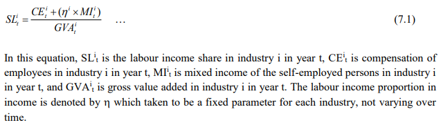 The derivation of the GVA series for different industries has been briefly explained in Chapter 2. The derivation of CE and MI series has been explained in step I above. Therefore, only the estimation method of η needs to be described. The estimation of η has been done with the help of NSS survey-based estimates of employment of different categories of workers (number of persons and days of work) and wage rates (which has been described briefly in chapter 4) coupled with estimates of MI, basically obtained from the NAS. Two approaches have been taken to get an estimate of η, and the labour income share series for different industries finally adopted in the study makes use of an average of the estimates of η obtained by the two approaches. In the first approach, an estimate of labour income of self-employed workers has been made for each study industry for eight years, 1983-84, 1987-88, 1993-94, 1999-00, 2004-05, 2009-10, 2011-12 and 2015-16 on the basis of the estimated number of self-employed, wage rate of self-employed and the number of days of work per week. The industry-wise estimates of number of self-employed, wage rate of self-employed and the number of days of work per week have been made from unit records of NSS employment-unemployment survey (major rounds) of 1983, 1993-94, 1999-00, 2004-05, 2011-12, and PLFS from 2017-18 onwards. The estimates of the number of self-employed, wage rate of self-employed and the number of days of work per week provide an estimate of the annul labour income of self-employed workers which is divided by the mixed income of self-employed (derived from NAS) to get an estimate of η. For five industries, the ratio in question has been computed and applied. For the other 22 industries, the ratio in question has been computed after clubbing the industries into 11 industry groups.21 In the latter case, a common ratio computed for group of industries has then been applied to constituent industries. The list of industries or industry groups for which η has been estimated is given in Table 7.2. In the second approach, the NSS data are used to compute the following ratio: the ratio of labour income of self-employed workers to the labour income of regular and casual workers. Let this be denoted by θ. Then, the estimate of CE provided in the NAS is multiplied by θ to obtain an estimate of the labour income component out of the MI reported in the NAS. The labour component of MI divided by total MI gives an estimate of η. In case the estimated labour component of MI exceeds the estimate of MI, the estimate of η has been taken as unity. Examining the estimates obtained by the first approach, it was found that the estimated labour income share out of mixed income varied significantly among the estimates for the seven years for which the ratio in question has been estimated. The estimates of η obtained by the second approach has the problem that in a number of cases, the estimated labour component of MI exceeds the estimate of MI given in the NAS, and therefore η is taken as one. The method finally adopted is as follows: (a) The average value of η has been computed for each industry or industry group by taking the estimates for the years 1983-84, 1987-88, 1993-94, 1999-00, 2004-05, 2009-10, 2011-12 and 2015-16. This has been done separately for the estimates based on approach-1 and those based on approach-2. (b) The estimates of η obtained for each industry or industry group by the two approaches have then been averaged. (c) Having obtained an estimate of η, equation 7.1 given above has been applied to compute the labour income share. Construction of Factor Income Share Series in Gross output The income share of labour, capital and intermediate inputs in Gross output has been computed using the following steps:
The splitting of unorganized sector factor incomes into individual industries has been done using unorganized survey results. The proportions computed for 1983-84 has been applied for the period 1980-81 to 1983-84. While there were surveys of unorganized manufacturing enterprises in 1978-79 the survey results have not been used for estimation of factor incomes in different industries of the unorganized manufacturing sector. Chapter 8: Growth Accounting Methodology
This chapter deals with the methodology of measurement of total factor productivity (TFP) growth for individual industries in the KLEMS framework and the aggregation from industry level productivity measures to measures for broad sectors and the economy as a whole. The methodology of analysis of sources of gross output growth at the individual industry level and sources of GVA (Gross Value Added) or GDP growth at the broad sector level and economy level will also be presented in this chapter 8.1 Methodology for Measuring Productivity Growth at the Industry level The production function Our measurement of TFP growth for different industries of the Indian economy is based on a gross output production function for each industry j:  Y is industry gross output, L is labour input, K is capital input and E, M and S are intermediate inputs-namely energy, material and services and T is an indicator of technology for industry j. All variables are indexed by time (t subscript is suppressed). There are several things to note about the production function - (1) all variables are aggregates of many components that have been discussed in the earlier report/chapters; (2) we assume that the industry production function is separable in these aggregates; (3) time (indicator of technology) enters the production function symmetrically and directly with inputs. An important feature of the gross output approach is the explicit role of intermediate inputs. In our study, we have considered three intermediate inputs - energy, material and services and this is important as we may find that intermediate inputs are the primary component of some industries outputs22. Failure to quantify intermediate inputs leads us to miss both the role of key industries that produce intermediate inputs and the importance of intermediate inputs for the industries that use them. To estimate the contributions of total factor productivity, and inputs to industry level output growth, based on the above-mentioned production function, we construct real values of inputs and output, using industry level price data for capital, labour and intermediate inputs, and output. e.g., PYj; PLj, PKj; PEj. PMj, PSj. The industry price of an input varies across industries due to compositional effects as industries expend different shares of their investment on each type of asset. The same is true for all inputs. Total Factor Productivity To estimate TFP growth, we begin with the fundamental accounting identity for each industry where the value of output equals the value of inputs. 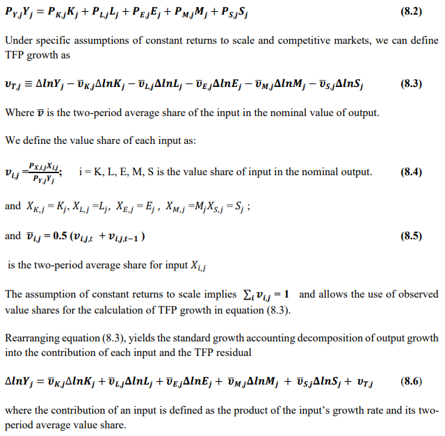 We can further decompose the contribution of each input into a quantity and quality component. As discussed earlier, the quality component represents substitution between H components, while the quantity component represents the increases in each detailed input. Our extended decomposition of the sources of output growth is given as follows:  Where Z is the stock of industry capital, Qk is the capital quality, H is number of persons employed and Ql is the quality of labour. The data series at individual industry level constructed for gross value added and gross output, labour input, capital input, intermediate inputs and factor income shares (described in Chapters 2, 3, 4, 5, 6 and 7, respectively) are used to estimate TFPG during the period 1980 to 2019. Labour input is measured by using total person worked along with the labour quality index (see Chapter 4 for a detailed discussion). The series on growth rate in capital services forms the measure of growth in capital input (discussed in Chapter 5). TFPG estimation is done by using the gross output function framework23 (i.e. equation 8.7). 8.2 Methodology for Aggregation across Industries We also provide the TFPG for aggregate economy and two broad sectors, viz. manufacturing and services24. However, the method of estimation of TFP growth for individual industries described in section 8.1 cannot be readily applied to a higher level of aggregation. The main problem is that gross value of output cannot be added across industries to generate a measure of output at a higher level of aggregation, say for the economy or of any of the broad sectors. Therefore, it becomes necessary to consider appropriate methods of aggregation across industries consistent with the gross output function specification of technology at the individual industry level. We use the Törnqvist index25 for aggregating across the broad sector and total economy. Taking this approach, computations are made for the manufacturing sector, the services sector, and for the aggregate economy. These aggregates are obtained using Törnqvist aggregate of growth rates of real value added, capital input, and labour input. Below, we briefly describe the Törnqvist index. Suppose the aggregate sector J consists of n KLEMS industries (j=1:n). We obtain the output (vale added) and inputs aggregates for sector J as: 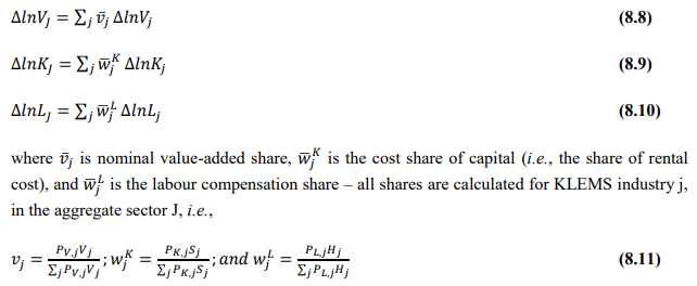 where PV,j is the price of value added in industry j, Vj is the real value added in industry j, PK,j is the rental price of capital in industry j, Sj is the capital stock in industry j, PL,j is the wage rate (price of labour) in industry j, and Hj is the employment in industry j. The aggregate output (real value added) and input growth rates obtained above are then used with the growth accounting equation to obtain the sectoral TFP growth rates. 1 From both aggregated 9 NAS sectors Gross Domestic Product by economic activity statement along with the disaggregated statements of these 9 NAS sectors. 2 In the EUS, the persons employed are classified on the basis of their activity status into usual principal status (UPS), usual principal and subsidiary status (UPSS), current weekly status (CWS) and current daily status (CDS) for quinquennial rounds. UPSS refers to a person’s employment status based on what he/she might have been engaged in over a period of 365 days preceding the date of survey. 3 See Table 7 on pg. no 371 of Economic Survey 2021-22, Government of India (https://www.indiabudget.gov.in/budget2022-23/economicsurvey/doc/echapter.pdf). 4 See Table 8 on pg. 44 on https://main.mohfw.gov.in/sites/default/files/Population%20Projection%20Report%202011-2036%20-%20upload_compressed_0.pdf 5 This is also the mid-point of financial year. 6 For more detailed discussion on extrapolation and interpolation of the series, readers may refer to KLMES data manual version 2022 released by RBI on its website. 7 In PLFS, the earnings by self-employed are also provided, but for consistency with other rounds we have used the same procedure of Mincer equation even for this round. In EU KLEMS (Timmer, et.al., op cit; p 67) it is assumed that the earnings of the self-employed is equal to the earnings of ‘regular' employees. 8 For detailed explanation of Heckman two-step process, one may refer to the previous year manual 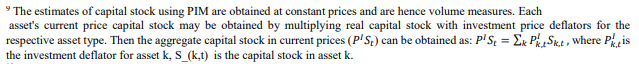 10 This version of the database does not make a distinction between ICT and non-ICT assets, as the industry level data on ICT assets are weak. An attempt to estimate aggregate economy level ICT capital can be found in Erumban and Das (2015). 11 See O’ Mahony and Timmer (2009) for a description of EU KLEMS database 12 This data is not publicly available. However, CSO has been kind to compile this data for the India-KLEMS project. 13 In some years transport equipment was provided as part of the machinery and equipment, categorized as ‘tools, transport equipment and other fixed assets. In such cases, we use transport/tools, transport and other fixed asset ratio in the nearest year to separate transport equipment. 14 A detailed discussion on how the series prior to 2011-2012 were adjusted to match the subsequent series is provided in Box 5.2A in the Appendix. 15 Gross investment is estimated as the difference between book value of asset in period t and in period t-1 and add depreciation in period t to that. 16 This choice is driven by the fact that the first year of availability of ASI data is 1964-65. 17 National Accounts Statistics-Sources and Methods, Chapter 26, CSO (2007), 18 We do not intend to delve into the controversies over the use of internal vs. external rate of return in the context of productivity measurement. This database uses See Erumban (2008a and b) for a discussion on these issues. 19 Reserve Bank of India, Handbook of Indian Statistics, Annual volumes. 21 The estimation is done at group level rather than individual industries on the consideration that the group level estimates will be more reliable. 22 Consider, the semi-conductor (SC) industry, which is a key input to the computer hardware industry. Much of the output is invisible at the aggregate level because semi-conductor products are intermediate inputs to other industries rather than deliverables to final demand - consumption and investment goods. Moreover, SC plays a role in the improvements in quality and performance of other products like-computers, communication equipment and scientific instruments. Failure to account for them leads us to miss the role of key industries that produce intermediate inputs and importance of intermediate inputs for the industries that use them. (Jorgenson, Ho and Stiroh (2005), Productivity, volume 3). 23 It should be pointed out that an alternate set of estimates of TFPG obtained by using the value-added function framework is also provided in the India KLEMS dataset for which real gross value added is taken as the measure of output and only the two primary inputs are considered, namely labour input and capital input 24 More sophisticated methods of aggregation, such as the application of production possibility frontier approach or the application of direct aggregation is done in research papers written on the basis of the KLEMS dataset prepared. Such estimates of TFP growth are not a part of the database. 25 There exists other approaches to aggregate across broad sectors and industry, a detailed discussion on them can be found in KLEMS data manual version 2020 released by RBI on its website |
|||||||||||||||||||||||||||||||||||


Estimates of Productivity Growth for the Indian Economy
|
There is a major data gap in terms of availability of a consistent series on productivity for the Indian economy, though many individual researchers have estimated productivity for different sectors and the overall economy for specific time periods using different methodologies. In order to address this data gap, the Reserve Bank had funded a project in the Indian Council for Research on International Economic Relations (ICRIER) on productivity measurement following the EU-KLEMS (Capital, Labour, Energy, Material and Services) methodology. The research work under the project was carried out by a team comprising Dr. Deb Kusum Das, Professor Suresh Aggarwal, Dr. Abdul Azeez Erumban, Ms Sreerupa Sengupta, Ms Kuhelika De and Shri Pilu Chandra Das under the overall guidance of Professor B. N.Goldar. The team was also guided by an Advisory Committee under the chairmanship of Professor K.L.Krishna and with Dr. Isher Ahluwalia, Prof. K.Sundaram, the late Prof. Suresh Tendulkar, Dr. Ramesh Kolli, Prof. T C Anant, Dr. R.Radhakrishna, Prof. Dale Jorgenson, Prof. Marcel Timmer, Dr. Bart Van Ark, Prof. Mary O’Mahony and the undersigned as members. The research team has since submitted three reports delineating the methodology of productivity measurement in the KLEMS framework and estimates of productivity growth along with the time series data for the period 1980-81 to 2008-09. With the objective of making this data and methodology available to the broader community of researchers and analysts, the current Report on “Estimates of Productivity Growth for the Indian Economy” is being released by the Reserve Bank of India. The abridged version of the Report, based on the original three Reports, has been prepared by an internal team of officers led by Smt. Balbir Kaur and comprising Shri Rajib Das, Smt. Sangita Misra, Shri Alok Ghosh, Ms Alice Sebastian and Shri Anoop K. Suresh. The Reserve Bank of India takes this opportunity to thank ICRIER and the research team for this useful endeavour, the Advisory Committee for their guidance and all those, both within the RBI and outside, who have contributed to the project in different ways. It may, however, be emphasised that the data on productivity and related analysis given in this report reflect the research output of the India KLEMS research team and, therefore, do not represent an official series on productivity by the Reserve Bank of India. Given the enormous data challenges and differences in methodology in this area, the researchers may ensure adequate caution in the use of the data. Deepak Mohanty Research Advisor Team Members The Report titled “Estimates of Productivity Growth for Indian Economy” presents the work carried out by the India KLEMS project at ICRIER in collaboration with the Reserve Bank of India. The research project has computed a time series database on productivity growth for the Indian economy and has, thus, tried to fill in an important data gap in this area. Some of the distinguishing features of the project are described below:
Some of the major findings of the Report are outlined below:
As regards labour productivity, the median growth for the economy as a whole was observed to be 4.1 per cent during 1980-2008, with higher growth rates in manufacturing industries, the electricity sector and certain services. When it comes to the growth rates of various inputs, labour input (Index of persons employed multiplied by index of labour composition) grew the fastest in construction and some service industries, while the agriculture sector remained a laggard. The growth rate of capital services in the economy was 6.5 per cent per year. It was the highest at 8.8 per cent in the broad sector of manufacturing and the lowest at 3.5 per cent in the agriculture sector. As regards the trend rates of growth for intermediate inputs, enormous heterogeneity is observed across industries in the range of 12.8 per cent (for post & telecommunication) to 2.3 per cent (for agriculture). The findings of this research project confirm the dominant role of input accumulation vis-à-vis productivity growth in explaining India’s economic growth. Productivity Growth is studied extensively because it is a contributory factor in the improvement of living standards. In recent years, leading researchers in productivity have turned their attention to the measurement and analysis of productivity at the disaggregate industry level that covers the entire economy of selected countries. While much of the earlier research was based on a value added version of the production function, ignoring the explicit role of intermediate inputs in the production process, recent work on productivity for several countries has been based on the Gross Output version of the production function for all individual industries comprising the economies. It is against this backdrop that the KLEMS research project was undertaken in September 2009 with two major objectives:
The KLEMS research project has computed productivity growth estimates through two different approaches: (1) using a value added production function, incorporating labour and capital inputs for the Indian economy and for 26 sectors for the period 1980-2008 and (2) gross output methodology of computing productivity and incorporating primary inputs of capital (K) and labour (L) along with the intermediate inputs of energy (E), materials (M) and services (S). In estimating productivity growth, the quality aspects of two inputs—labour and capital—have been explicitly addressed. Two dimensions of the labour input were distinguished—labour persons and educational attainment of the workforce—so that the contribution of education to value added growth at the individual industry level could be assessed. With regard to capital input, three asset types were distinguished: (i) construction (structures), (ii) transport equipment and (iii) machinery and equipment. Taking into account the differences in the length of life (depreciation) of the three asset types, measures of capital services were derived for each sector/industry. For measurement of capital input for the economy as a whole, ICT capital was also taken into account. Along with the productivity estimates, the project has also generated new datasets on labour, capital and the three intermediate inputs—energy, material and services—for each of the years over the time period that allow greater accuracy in the estimation of productivity growth at the industry level as well as the economy and its broad sectors. The database for the study is prepared for use in the growth accounting methodology for estimating total factor productivity. Growth accounting allows a decomposition of output growth into the contribution of the different inputs and total factor productivity. The period covered is from 1980-81 (1980) to 2008-09 (2008). The industrial classification used for the study is along the lines of EU KLEMS1 so as to ensure comparability with other studies under the KLEMS project, where each economy is divided into 26 industries, as shown in Table 1.1. (In particular, the input-output (IO) tables could be aggregated to only 26 industries.)
The industrial classification was constructed by building concordance between NIC2 2004, NIC 1998, NIC 1987 and NIC 1970 so as to ensure continuous time series from 1980 to 2008. The database for 26 industry disaggregation consists of Agricultural sector (1), Mining and Quarrying sector (1), Manufacturing industries (13), Electricity, Gas and Water supply (1), Construction (1) and Services sector (9) comprising both market and non-market services. Measures of capital (K), labour (L), energy (E), material inputs (M) and service inputs (S) as well as gross output (GO) and value added (VA), were constructed using National Account Statistics (NAS), Annual Survey of Industries (ASI), NSSO rounds and input-output (IO) tables. For certain industries, annual data from NAS and ASI were used to compute time series on gross output. However, NSSO rounds of unregistered manufacturing, Employment and Unemployment Surveys by NSSO and input-output tables are available only for benchmark years. This necessitated interpolation and assumption of constant shares for construction of time series for gross output (unregistered manufacturing, services sector), intermediate inputs and labour inputs. An overview of earlier productivity research in India is attempted in Chapter 2 to provide a background on both issues and methodologies that have been addressed in past studies. The Indian literature on productivity measurement is quite vast. In Chapter 3, the methodology for computing total factor productivity (as well as labour productivity) growth rates at the industry, sector and economy levels is discussed. The chapter outlines three different aggregation procedures for arriving at the economy-level productivity growth rates. The different sources used for the construction of data series and the methodology adopted for the construction of both value added and gross outputs series are explained in Chapter 4. The various sub-sections of Chapter 5 outline the methodology adopted for the construction of labour input, capital input and intermediate inputs—energy (E), material (M) and services (S). The productivity growth estimates derived using the compiled data series on gross value added, gross output, labour, capital, and Intermediate inputs are presented in Chapter 6. Chapter 7 discusses estimates of labour productivity and total factor productivity growth for six broad sectors and the economy. Chapter 8 presents a summary of the findings and conclusions derived from the study. Chapter 2: Overview of Productivity Research in India The Indian literature on productivity measurement is quite vast, and is growing fast. The quality of research has improved steadily over the years. While the bulk of the past productivity research has been on the manufacturing/ industrial sector (Ahluwalia, 1985, 1991; Goldar, 1986, 2004), there have been several studies on productivity growth in agriculture and services, and the economy as a whole. The Indian productivity literature, particularly the studies on manufacturing, has been reviewed by Goldar (2011b), Goldar and Mitra (2002) and Krishna (1987, 2006, 2007), among others. This chapter presents a brief overview. 2.2 Productivity in manufacturing Chronologically, productivity studies on Indian manufacturing can be divided into three groups. The first generation studies, which include the studies undertaken by Reddy and Rao (1962), Banerji (1975), Goldar (1986) and Ahluwalia (1985), came up with estimates of TFP growth that indicate that TFP growth in Indian manufacturing in the period 1951 to 1979 was slow or negative. The second-generation studies drew attention to the biases in productivity estimates arising from the use of value added function and particularly the use of single deflated value added. Two prominent studies belonging to this group are Balakrishnan and Pushpangadan (1994) and Mohan Rao (1996). These studies contested the assertion made by Ahluwalia (1991) that there was a marked acceleration in TFP growth in manufacturing after 1980 which was attributed to liberalisation of economic policies. Ahluwalia had relied on the single‐deflation (SD) procedure. The more appropriate double‐deflation (DD) procedure by Balakrishnan and Pushpangadan resulted in TFPG estimates that contradicted Ahluwalia’s claim. Mohan Rao’s results based on (i) double deflation in the case of value added production function and (ii) gross output production function as well as those of Pradhan and Barik (1998) using the Gross Output function lend support to the contention of Balakrishnan and Pushpangadan that there was no turnaround in productivity growth in manufacturing in the 1980s3. The third-generation studies have mostly focussed on the impact of industry and trade policy reforms on industrial productivity growth in the post‐reform period (i.e., the period since 1991). The third-generation studies have, in most cases, used the gross output function for the measurement of TFP. These studies take services as an input along with capital, labour, materials and energy to estimate total factor productivity growth in Indian manufacturing. The overall conclusion one may draw from the findings of these studies is that there has been no improvement in the rate of TFP growth in Indian manufacturing in the post‐reform period compared to the growth rate achieved in the 1980s. Rather, TFP growth has slowed down. Trivedi et al (2011) for instance report that the TFP growth rate in manufacturing was 1.88 per cent per annum during 1980 to 1991 and 1.05 per cent per annum during 1992 to 2007. As regards the unorganised manufacturing sector, there have been only a couple of productivity studies. Most of them report a downward trend in TFP (Prakash (2004), Unni et al. (2001), Kathuria et al. (2010)). 2.3 Productivity in Agriculture Estimates of TFP growth are available for aggregate agriculture, crop sector, livestock sector and even individual crops such as rice, wheat, maize and sugarcane. Estimates have also been worked out at the state level for major crops. Concerns have been expressed on the basis of available evidence that agricultural growth is becoming unsustainable as a result of resource (soil) degradation. Mukherjee and Kuroda (2003) report that the growth rates in TFP in Indian agriculture were 1.45 per cent per annum during 1973‐80, 2.33 per cent per annum during 1981‐88 and 1.21 per cent per annum during 1989‐93. Between 1973 and 1993, the average rate of growth in TFP was 2.02 per cent per annum. There have been several productivity studies on specific sub‐sectors of services. The Indian Railways, for example, has been studied by Sailaja (1988) and Alivelu (2006). Similarly, productivity in Indian airlines has been studied by Hashim (2003), productivity in the insurance industry by Sinha (2007), and productivity of the information technology industry by Mathur (2007). In comparison with other sub‐sectors of services, a much larger number of studies on productivity and efficiency have been undertaken for banks, e.g., De (2004) and Sinha and Chatterjee (2008). The estimates of TFP growth presented in two studies (Goldar and Mitra 2010; Virmani, 2004) indicate that there was a marked acceleration in TFP growth in services after 1980 (Table 2.1).
2.5 Inter‐Sectoral Perspective Bosworth et al. (2007) present sources of economic growth during 1960‐2004, for the three sectors, namely, agriculture, industry and services, as well as the total economy. Going by their estimates (Table 2.2) the productivity performance of the services sector was the best in the sub‐periods 1960‐80 and 1980‐2004. Overall, the performance was unsatisfactory in all three sectors during the first sub‐period. The estimates of productivity presented in Bosworth and Maertens (2010) show a pattern very similar to that in Bosworth et al., (2007). The growth rate of TFP in services exceeded that in industry and agriculture in the periods 1980‐90, 1990‐2000 and 2000‐2005 (Figure 2.1). The gap in the TFP growth rates between services and other sectors was relatively greater in the period 1990 to 2000. A similar pattern is observed in the estimates of TFP growth in agriculture, industry and services reported by Verma (2008). Figure 2.1: Total factor productivity growth, India, by broad sectors of the economy  2.6 Productivity Studies for the Aggregate Economy Four major recent studies on sources of growth of the Indian economy are by Dholakia (2002), Sivasubramonian (2004), Virmani (2004), and Bosworth, et al. (2007)4. Table 2.3 shows the estimates of TFP growth for the aggregate economy obtained in various studies. The broad conclusion one may draw from the productivity growth estimates presented in the studies is that the rate of TFP growth in the Indian economy accelerated sharply after 1980. Also, there is an indication that the rate of growth in TFP in the post‐reform period has been higher than that achieved in the 1980s. The acceleration in TFP growth at the aggregate economy level seems to be rooted in the improved productivity performance of the services sector.
2.7 Attempted Improvements in the Present Study The present study attempts to improve on the past productivity research in India on several counts. While the majority of the previous studies were concerned with a sector or a sub-sector of the economy, the present study has comprehensive coverage. Arguably, studies undertaken by Virmani (2004) and Bosworth et al. (2007) also have comprehensive coverage, but they have not divided the economy into as many sub-sectors or industries as done here. The second advantage of the present study is that the industrial classification and the methods of measurement of output and inputs have been chosen so as to render international comparability of the productivity estimates. This will make it possible to validate international comparisons of productivity growth for a large number of sub-sectors or industries in India. In this regard, several earlier studies have a handicap. The third point is that careful attention is paid in this study to the measurement of inputs, labour and capital. The measure of labour input takes into account the educational characteristics of the workforce. While some earlier studies have also taken into account changes in labour quality, this has by and large been ignored in the past productivity research in India. As regards capital input, an attempt is made to estimate capital service rather than use capital stock as all earlier studies in India have done. The measurement of capital services is done by taking into account the changing composition of capital assets and also the growing use of information and communication technology (ICT) in the Indian economy. This greatly improves the measurement of capital input and helps obtain a more accurate measure of total factor productivity growth. Chapter 3: Methodology of Productivity Measurement in the KLEMS Framework: This chapter deals with the methodology for measurement of total factor productivity (TFP) growth for individual industries in the KLEMS framework and the aggregation from industry-level productivity measures to measures for broad sectors and the economy as a whole. The methodology for analysis of sources of gross output growth at the individual industry level and sources of GVA (Gross Value Added) or GDP growth at the broad sector level and economy level will also be presented in this chapter, which supplements the discussion on these aspects in Chapters 6 and 7. 3.2 Measuring Productivity Growth for Individual Industries The methodology developed by Jorgenson and his associates and presented in Jorgenson et al. (2005) is adopted. This methodology has been followed recently in Timmer et al. (2010) for the European Union and the US. Let the production function for industry j be denoted by where Y is industry gross output, K is capital input, L is labour input, E is energy input, M is material input and S is services input, and T is an indicator of technology, all for industry j. All variables vary over time t, but the t subscript is not shown explicitly, for the sake of simplicity. For the calculation of total factor productivity (TFP) growth, the accounting identity for each industry is taken into account: The identity states that the value of gross output of industry j equals the sum of the values of the five inputs.PY denotes the price of output, PK,PL,PE,PM and PS are the prices of capital, labour, energy, material and services, respectively. The identity implies constant returns to scale. Assuming that the five input markets are competitive and factors are paid their marginal products, gross output TFP growth AjY for industry j can be obtained as:   The sources of labour productivity growth are change in capital intensity, change in labour composition and TFP growth, as shown in (3.18). 3.3 The Industry Origins of Aggregate Grow To use measures of individual industries to arrive at aggregate measures for broad sectors and the economy, Jorgenson et al. (2005) consider three alternative approaches to aggregation. Approach I is based on the existence of the aggregate production function, for which four key assumptions are necessary. These assumptions are very restrictive and unrealistic. In this approach aggregate value added is simply the sum of value added for the constituent industries. Approach II is based on the existence of the Aggregate Production Possibility Frontier. The most restrictive assumption of production function being the same for all industries is relaxed. Aggregate value added is given by the Tornqvist formula:  PjV being the price of value added for the jth industry. Aggregate capital input and labour input are also given by the Tornqvist formula. Approach II is preferred to Approach I. Approach III: Direct Aggregation across Industries This method was developed by Jorgenson, Gollop and Fraumeni (1987). Jorgenson et al. (2005) and Timmer et al. (2010) have applied this approach in their respective studies. Labour Productivity (δ) is defined as value added per person employed, i.e., Z/N. As shown by Stiroh (2002), aggregate labour productivity can be decomposed into industry contributions as follows:  This formula enables us to determine the contribution of capital deepening, labour composition and TFP growth from each industry to aggregate labour productivity growth. The decomposition of the growth of gross output of industry j is given by where Xj refers to intermediate inputs   Chapter 4: Database for Gross Value Added and Gross Output This chapter describes the procedures used to construct the database for gross output and value added series at the industry level over the period 1980-81 (1980) to 2008-09 (2008). Both the raw data sources and the adjustments that have been made to generate the comprehensive time series on output and value added are consistent with the official National Accounts. Multiple sources of information are used for the construction of the database on gross output and gross value added. The main sources of data are the National Accounts Statistics (NAS), Input-Output transaction tables (IOTT), Annual Survey of Industries (ASI) and the follow-up surveys of unorganised manufacturing conducted by the NSSO, Office of the Economic Adviser, Ministry of Commerce and Industry. The details of the construction of various variables from these data sources are discussed in different sections of the chapter. This chapter is divided into two sections. Section 4.2 documents the data sources and methodology for constructing the Gross Value added (GVA) series. Similarly, Section 4.3 describes the data sources and methodological details for estimating the Gross Value of Output (GVO) series. It also presents the trend growth rates and value added shares of GVA for the study period 1980 to 2008 and the empirical estimates (trend growth rates at industry level) of the GVO series for the period under study. 4.2 Gross Value Added: Data Sources and Methodology Gross value added of a sector is defined as the value of output less the value of its intermediate inputs. Value added created by a sector is shared between labour compensation and capital compensation. The growth rates of gross value added for the total economy determines the rate at which the Indian economy is growing. The trend growth rates of gross value added in different industries determines the pace at which that industry is growing relative to the total economy. 4.2.1 Data Sources for Gross Value Added The National Accounts Statistics (NAS) brought out by the CSO is the basic source of data on gross value added in India. NAS has provided estimates of GDP (i.e., gross value added) by industry of use at both current and constant (1999-2000) prices since 1950 at both aggregate and disaggregated levels. The sectors for which data are provided in NAS are Agriculture, Forestry & logging, Fishing, mining & quarrying, Manufacturing (registered and unregistered), Electricity, Construction, Trade, Hotels & Restaurants, Railways, Transport by other means, Storage, Communication, Banking & insurance, Real estate, Ownership of dwelling & business services, Pubic administration & defence and Other services. Further, NAS provides estimates of GDP at the disaggregated level for these industries. The data on GDP for the manufacturing sector at the more disaggregated levels are available in the ASI and NSSO quinquennial surveys for registered and unregistered manufacturing industries, respectively. These data sources are used to construct value added series for 26 industries for the period 1980 to 2008. It is to be noted that gross value added at current and constant prices has been constructed using the NAS back series, i.e., NAS 2009 and NAS 2011. The new data from NAS 2011 (2004-05 base) is linked with the old NAS 2009 data (1999-2000 base) through splicing to update the estimates for the period 2004 to 2008. Growth rates of the old series (1999-2000 base) are applied to the level of the new series (2004-05 base) with 2004-05 as the link year. 4.2.2 Methodology for Construction of Gross Value added Series The concordance of NAS sectors and 26 industries was identified, as the first step for construction of the value added series. In India, output is adjusted for Financial Intermediation Services Indirectly Measured (FISIM). The value of such services forms a part of the income originating in the banking and insurance sector and is deducted from the GVA. The NAS provides output net of FISIM for some industry groups at the aggregate level. For instance, in the estimates of GVA obtained for the registered manufacturing sector, adjustment for FISIM in NAS is made only at the aggregate level in the absence of adequate details at a disaggregated level. However, FISIM have been allocated to all the manufacturing sectors by redistributing total FISIM across sectors proportional to their sectoral GDP shares. Similar redistribution of FISIM has been done for the trade sector and the other services sector. For manufacturing industries where direct estimates of GVA are not available from NAS, estimates have been made using additional information from ASI and NSSO unorganised manufacturing sector data. To obtain the estimates of GVA for registered manufacturing industries, data from the ASI based on the National Industrial Classification 1998 (NIC-1998) obtained from the Economic and Political Weekly electronic database have been used. For the unregistered manufacturing sector, results from five rounds of NSSO surveys—40th round (1983-84), 45th round (1989-90), 51st round (1994-95), 56th round (2000-01) and 62nd round (2005-06)— have been used to obtain value added estimates. In India, the estimates of GVA for the unregistered manufacturing sector are obtained as a product of the work force and the corresponding GVA per worker. Information about employment in the unorganised sector is only available in the benchmark years for which NSSO survey data are available. Therefore, there is no consistent source of employment data for the years between these quinquennial surveys. The information on value added per worker is equally limited, since the value added data are updated at approximate 5-year intervals (for details, see CSO, 2007). Therefore, estimates of value added for the unregistered manufacturing sectors for the years between the benchmarks have been obtained by interpolation as well as by extrapolation. For 19 of the 26 industries listed in Table 4.1, GVA series both at current and constant prices are directly available in NAS. GVA data series at current prices for the remaining 7 study manufacturing industries are constructed by splitting the data of 7 NAS industries using additional information from ASI and four NSSO surveys. Once the nominal estimates of GVA of 7 manufacturing industries are obtained, the current price estimates are deflated using suitable WPI deflators to arrive at constant price series. To maintain consistency with NAS, the study has proportionately adjusted the deflated figures of 7 manufacturing industries with overall estimates of GVO of 7 NAS manufacturing industries. It is worth noting that our aggregate estimate of GVA in manufacturing (formed from using the shares of ASI data and NSS unorganised manufacturing surveys) is consistent with the overall estimate of gross value added in NAS. As mentioned earlier, the current and constant price series of the remaining industries are directly taken from NAS. 4.2.3 Value Added Shares One of the most interesting features of the Indian economy since the 1980s is the emergence of services as the dominant sector and as the main driver of GDP growth. Looking at the percentage distribution of value added share, it is evident that the services sector had the highest share in all three years. Among the 9 services sectors, trade, other services, transport & storage, public administration & defence and financial services had high value added shares in all three years. For the manufacturing sector, there is a slight fall in value added share from 1980 to 2008. Though agriculture has been the second largest contributor (after the services sector) to India’s GDP over the years, its share has sharply declined from 36 per cent in 1980 to 18 per cent in 2008. The share of value added of construction increased sharply from 4.6 per cent in 1980 to 8.1 per cent in 2008, while that of the services sector increased from 40 per cent in 1980 to 54 per cent in 2008. 4.2.4 Trend Growth Rate of Real Gross Value Added for 26 sectors of the Indian economy The individual trend gross value added growth for 26 industries for the period 1980-2008 have been estimated using the exponential model for growth estimation. Table 4.1 also documents the trend GVA growth of 26 industries during the period covered. 4.3 Gross Output: Data Sources, Methodology and Estimates The gross output of an industry is defined as the value of production using primary factors such as labour, capital and intermediate inputs purchased from other industries. As per the growth accounting methodology, the gross output of each industry is a function of capital, labour, intermediate inputs and technology. An important advantage of gross output approach is that it provides a complete measure of production and treats all inputs—labour, capital and intermediate inputs—symmetrically. In contrast, the value added measure of output does not explicitly account for the flow of intermediate inputs that may be the primary component of an industry’s output. 4.3.1 Data Sources for Gross Output NAS, published by the CSO, is the basic source of data used to construct the gross output series of various sectors at current and constant prices. For industries where NAS does not provide direct estimates of output, additional information is used from the ASI for registered manufacturing sectors, NSSO quinquennial surveys for unregistered manufacturing sectors, and input-output transaction tables for service sectors. As in the value added case, the required splicing is done to get a comparable time series. 4.3.2 Methodology for Construction of Gross Output Series i) Current Price series Concordance between NAS industries and our 26 study industries is the first step in the construction of the output series. NAS provides nominal GVO series for a) crops and plantation, b) animal husbandry, c) forestry and logging and d) fishing. By aggregating the GVO of these four sub-sectors, the output of the agriculture sector is derived. For manufacturing industries, time series on gross output is obtained by adding the magnitudes for registered and unregistered segments of manufacturing. As mentioned earlier, NAS estimates of gross output for manufacturing industries are at a more aggregate level. In such cases, the aggregate output of NAS at current prices has been split using additional information from ASI and NSSO unorganised sector reports. Gross output data both at current and constant prices for 6 of the 13 manufacturing industries are directly picked up from NAS. For the remaining 7 industries, output is constructed by splitting the NAS output data using ASI or NSSO distributions.ASI data (annual) has been used for registered manufacturing, whereas interpolated ratios from the NSSO 56th round (2000-01) and 62nd (2005-06) round have been used for the unregistered manufacturing sector. For the period prior to 1999, separate output estimates for the unregistered manufacturing sector are not available in NAS. Thus, to derive the output estimates for the time period 1980 to 1998, GVA to GVO ratios are computed from NSSO survey reports of the 40th round (1984-85), 45th round (1989-90) and 51st round (1994-95). The GVA to GVO ratio for the year 1999 is directly picked up from NAS. The ratios obtained are then linearly interpolated between intermediate years and applied to time series of GVA from NAS at current prices to obtain the output estimates at current prices. The ratios of the NSSO 40th round are taken backwards to derive output numbers for the period 1980 to 1983. Gross output series for services sectors and electricity, gas & water supply have been constructed using information from the IOTT of the Indian economy published by the CSO. The GVO to GVA ratios for services sectors are obtained from IOTT benchmark years of 1978-79, 1983-84, 1989-90, 1993-94, 1998-99 and 2003-04. These ratios are linearly interpolated for the intervening years and applied to the GVA series of NAS to derive output estimates consistent with NAS at current prices. It is to be noted that for the government-owned sector ‘Public administration & defence’ no intermediate inputs are given in the IOTT. Consequently, the value added to output ratio from the System of National Accounts tables have been applied to nominal GVA figures of NAS to estimate the output for this sector. Thus, a time series of gross output is constructed for 26 sectors at current prices. ii) Constant Price series Gross output series at constant prices for Agriculture, hunting, forestry & fishing, Mining & quarrying and Construction are directly available from NAS. For 6 of the 13 manufacturing industries, real GVO is taken from NAS. To arrive at constant price series for the remaining 7 industries, the study has deflated the nominal estimates with suitable WPI deflators. To maintain consistency with NAS, the study has proportionately adjusted the deflated figures with overall estimates of real GVO of 7 NAS manufacturing industries. Thus, our estimates of real GVO of total manufacturing exactly matches with NAS. For services and electricity, gas & water supply, the nominal estimates are deflated with implicit GVA deflators from NAS to arrive at constant price series. 4.3.3 Trend Growth Rate of Real Gross Output for 26 Industries of the Indian Economy The trend growth rate of gross output for each industry for the period 1980 to 2008 is estimated using the exponential model for growth rate estimation. Table 4.2 presents the trend growth rates of gross output of 26 KLEMS industries. For all 26 industries, the median growth rate of output was 6.9 per cent per annum. Output growth is found to be most rapid in post & telecommunications (14.2 per cent). Of the five fastest growing industries, two are producers of services (post & telecommunications and financial services) and three are manufacturing sectors (electrical & optical equipment, manufacturing nec, rubber & plastic products).All these industries posted growth rates in excess of 9.4 per cent during the period 1980 to 2008. The study also examines the trend growth rates of gross output and value added both at the aggregate and disaggregate levels of the economy for the period 1980 to 2008. It is observed that there is a strong positive correlation between real growth of output and real growth of value added. It is useful to highlight certain data issues related to measurement of output that are analogous to those explained in Jorgenson et al. (2005, Chapter 4) for the US economy and Timmeret al. (2010, Chapter 3) for the EU economy. The first basic measurement issue is that the annual GDP data are not consistent with the benchmark input-output tables from the official NAS. Second, there is a limitation in the estimation of gross output of electricity, since electricity produced for own use (both industries and households)/ captive power is not reported explicitly in the system of official statistics, whether ASI or other businesses. Third, the National Accounts does not provide any estimates of gross output of the services sector and, hence, the study relies on input-output transaction tables that are available at intervals of five years. This necessitates interpolation and assumption of constant shares for measuring output of services. This issue is analogous to that explained in Timmer et al. (2010) for the EU economy. Griliches (1994) paid particular attention to services sector output as a key source of uncertainty. Triplett and Bosworth (2004, 2008), in particular, concluded that in the US, output measurement in services has improved considerably, even as numerous areas for improvement still exist.
Chapter 5: Methodology and Database for Labour, Capital and Intermediate Inputs Multiple sources of information have been used for the construction of the database on labour input, capital input and intermediate inputs- energy, material and services. The main sources of data are the National Accounts Statistics (NAS), Employment-Unemployment Surveys (EUS) conducted by the NSSO, Input-Output (IO) tables, Annual Survey of Industries (ASI), the follow-up surveys of unorganised manufacturing conducted by the NSSO, and PROWESS data. These published data sources are supplemented by data especially furnished by the CSO for the project. 5.2 Labour Input – Data Sources, Methodology and Estimates Labour input is measured by combining data on labour persons and data on education. In the KLEMS framework it is desirable to estimate changes in labour composition by industries on the basis of age, gender and education. The measurement of labour composition is an attempt to distinguish one labour type from another, taking into account the embodied human capital in each person. The source of human capital could be through investment in education, experience, training, etc. The contribution to output by each person also comes from this embodied capital, and the reward (wages and earnings) to each person also includes the reward for investment in human capital. Therefore, it is essential to separate these differences in labour to clearly understand the underlying differences in labour characteristics. It is in this context that an endeavour has been made to estimate the labour composition index. However, given the limitations of India’s employment statistics, especially the non-availability of information on wages/ earnings of different categories of workers that could be used as an indication of differences in their ability, it is difficult to quantify these changes in the labour force in a pertinent way. The problems of employment statistics in India have been widely discussed in the literature (Himanshu, 2011; Sivasubramonian, 2004). This study aims to build a time series of employment data for 26 industrial sectors. However, there is no time-series data on the Indian economy, except for the organised segment. Therefore, it was essential to make certain assumptions regarding the annual changes in the employment series using the available information. 5.2.1 Data Sources and Methodology The section develops and implements the methodology of estimating labour input incorporating the indices of labour composition. Sources of data The Employment and Unemployment Surveys (EUS) by the National Sample Survey Office (NSSO) is the main source for estimating the total workforce in the country by industry group, as per the National Industrial Classification (NIC). The estimates obtained from the EUS are adjusted for population. The source of data for the population is the Census of India (different years), which only gives the decadal census; so, interpolated population is used for the intervening years. The study has used the unit-level data provided in the 38th (1983), 43rd (1987-88), 50th (1993-94), 55th (1999-2000), 61st (2004-05) and 66th (2009-10) major or quinquennial rounds of EUS that have been conducted by the NSSO since 1980. The 32nd major round (1977-78) has been used for extrapolating the labour series to 1980-81. In the EUS, the persons employed are classified on the basis of their activity status into usual principal status (UPS), usual principal and subsidiary status (UPSS), current weekly status (CWS) and current daily status (CDS) for quinquennial rounds. UPSS is the most liberal and widely used of these concepts and despite the fact that the UPSS has some limitations5, this seems to be the best measure to use given the data. Methodology
Efforts are made in this chapter to estimate persons employed industry-wise and adjust that measure for changes in labour skill by calculating the labour composition index, thus obtaining the composition corrected labour input. Since the NSSO used the NIC 1970 to classify persons employed by industry in the 38th and 43rd rounds, NIC 1987 for the 50th round, NIC 1998 for the 55th and 61st rounds, and NIC 2004 for the 66th round, as a starting point concordance between26 sectors and NIC-1970, 1987, 1998 and 2004 was done. Employment has then been computed as follows:
For extrapolation backward to 1980-81 to 1982-83, the interpolation of the broad industrial classification of the 32nd round (1977-78) and the 38th round (1983-84) is used. So the estimates from the 32nd round are mainly used as control numbers.
The composition of the labour force is of considerable importance in the context of productivity measurement, and a widely used methodology to capture changes in labour composition is given by Jorgenson, Gollop and Fraumeni (JGF) (1987). In growth accounting methodology, labour input is measured as an index of labour service flows. It accounts for changes in labour composition in terms of labour characteristics such as educational attainment, age or gender and, thus, accounts for heterogeneity of the labour force. In this method the aggregate labour input Lj of sector ‘j’ is defined as a Törnqvist volume index of persons worked by individual labour types ‘l’ as follows7:  where Δln Li,j indicates the growth of persons employed by labour type ‘l’ for sector ‘j’and weights are given by the period average shares of each type in the value of labour compensation, such that the sum of shares over all labour types is unity. It is assumed that the persons employed are paid their marginal productivities8 and since the study also assumes that marginal revenues are equal to marginal costs, the weighting procedure ensures that inputs that have a higher price also have a larger influence in the input index. Let Lj indicate the total persons employed in sector ‘j’ by all types Lj= Σ Li,j then the change in labour input (LI) can be decomposed as follows: The first term on the right-hand side, i.e., Δln LCj indicates the change in labour composition and the second term indicates the change in total persons employed in sector ‘j’. The index of aggregate labour composition, thus, measures the changes in the sex-age-education-occupation composition of the labour input in the economy. However, the use of this method is data-intensive. Due to data limitations of the sample size becoming very small as it is tried to estimate persons employed and earnings by industry by all the characteristics9, the present study has computed labour composition using only the education characteristic in the JGF methodology. For the labour composition index, the data required is employment by education by industry and earnings (compensation) for each cell. The labour composition index has been computed using five education categories10, namely, up to primary, primary, middle, secondary & higher secondary, and above higher secondary. There are, thus, five types of persons employed for each of the 26 study industries. It is estimated for the total persons employed in these industries in India for the 38th, 43rd, 50th, 55th, 61st and 66th rounds of the NSSO, with 1983 (38th round) equal to 100 so as to assess the temporal changes in labour skill. Since the series is required from 1980-81, the study has extrapolated it backwards from 1983 and interpolated between the major rounds. The composition index is recomputed with base 1980 as 100. Therefore, the following steps have been performed:
Second, earnings of the self-employed have also been estimated from the monthly consumption expenditure of these households. In this approach, first the total monthly consumption expenditure is divided by the number of employed persons in the household to get the total monthly consumption expenditure per employed person. Then, the ratio of wage earnings to total monthly consumption expenditure per employed person has been calculated for each industry by UPSS status. Assuming the consumption-earnings ratio to be the same for casual and self-employed persons, the ratio for casual labour is used for self-employed persons and this ratio is multiplied by the total monthly consumption expenditure per self-employed person to get the earnings of self-employed persons. However, if the earnings thus obtained are higher than the earnings obtained from the Mincer equation, then the latter are used. So, the lower of the two earnings- obtained from the Mincer equation or the earnings based on consumption expenditure- is taken to be the earnings of self-employed persons. It is to be noted that the two methods are used because they are based on i) household characteristics and ii) consumption expenditure. By combining the two, the study has moderated any upward bias in the estimation of wages for self-employed. Once the above steps are taken to find the educational distribution of all employed persons in all the six rounds and their corresponding wages, the labour composition index is computed14. 5.2.2 Trend Growth Rate of Labour Input for 26 Industries of the Indian Economy In this section, an analysis of the growth of the labour input is presented. The growth in persons employed and the labour composition for the entire period is given in Table 5.1. The growth rate of labour input (Index of persons employed multiplied by the index of labour composition) is summarised in Table 5.2. Growth of persons employed The rate of growth of persons employed is very different in different industries, reflecting a structural change during the period. For the full period the trend average growth of persons employed is 1.78 per cent. However, there have been changes in terms of employment growth in the Indian economy. While some sectors grew very fast, others remained stagnant during this period. Agriculture and mining & quarrying, which together employ the largest share of employed persons, has almost zero employment growth in the recent period. Consequently, their share in total employment has reduced from almost two-third to one-half. Among the sub-sectors of manufacturing it is found that very few sectors show rapid trend growth in employment. Construction is one important sector that has consistently experienced rapid employment growth. It has low labour productivity but vast employment potential and can be tapped for employment opportunities. Most sectors have registered a decline in the rate of employment growth in the recent decade15 except for textiles, wood, paper, transport equipment, hotels, construction and education and health. Growth of Labour Composition Index The growth in labour composition index is mainly the measurement of change in the educational skills of the employed persons over the period and their rewards for these skills. In India, the share of high-skilled labour (with education above higher secondary) has increased from a mere 2.4 per cent to almost 9 per cent. At the industry level, the growth in labour composition was the fastest in machinery, nec; chemical & products; other services; mining and quarrying; pulp & paper; and rubber & plastic products, but very slow in wood and products of wood; agriculture; basic metals and construction. Thus, the skill composition of each industry has changed differently over the period. The growth rate of labour input (index of persons employed multiplied by the index of labour composition) across industries is shown in Table 5.2. It reveals that labour input grew the fastest in post & telecommunications; machinery nec; construction; rubber & plastic products; other services and financial services. It is observed that the growth rates of labour input were higher than those of persons employed because of the contribution of labour composition. 5.3 Capital Input-Data source, Methodology and Estimat 5.3.1 Data Sources and Methodology As in the case of labour input where workers differ in terms of skill and experience, capital also consists of different vintages and asset types and these assets are not directly used in the production process; rather, the service delivered by these assets are the inputs to production. However, the empirical measurement of capital services is complicated due to the difficulty in quantifying the flow of capital services delivered by a unit of capital. Therefore, the usual practice is to assume proportionality between capital services and capital stock at the individual asset level (Hulten, 1986; Jorgenson, 1963; Jorgenson and Griliches, 1967). However, one should take account of the differences in the services delivered by different asset types, as each asset type differs in terms of its efficiency level. This would mean that even though one would assume proportionality between capital stock and capital service at the individual asset level, the weights differ across asset types and over time depending on the marginal productivity of each asset type16. Since marginal productivities are unobservable, one could, under neoclassical assumptions, approximate them by the prices of capital services delivered by each type of asset. Using this line of reasoning, Jorgenson (1963) and Jorgenson and Griliches (1967) have developed aggregate capital service measures that take into account the heterogeneity of assets. Using the Tornqvist approximation to the continuous Divisia index under the assumption of instantaneous adjustability of capital, capital services growth rate for asset type k is derived as a weighted growth rate of individual capital assets, the weights being the compensation shares of each asset, i.e.,  The rental price of capital Pk,tK reflects the price at which the investor is indifferent between buying and renting the capital good for a one-year lease in the rental market17. of taxation the rental price equation can be derived as under (see Christensen and Jorgenson, 1969; Jorgenson and Griliches, 1967): with it representing the nominal rate of return, δk the depreciation rate of asset type k, and Plk,t the investment price of asset type k. This formula shows that the rental fee is determined by the nominal rate of return, the rate of economic depreciation and the asset specific capital gains18. Ideally taxes should be included to account for differences in tax treatment of the different asset types and different legal forms (household, corporate and non-corporate). The capital service price formulas above should then be adjusted to take these tax rates into account. However, this refinement would require data on capital tax allowances and rates by industry and year, which is beyond the scope of this database. Available evidence for major European countries shows that the inclusion of tax rates has only a very minor effect on growth rates of capital services and TFPG (Erumban, 2008a). Since our measure of capital input takes account of asset heterogeneity, it was essential to obtain investment data by asset type. The study distinguishes between 4 different asset types -construction, transport equipment, non-ICT machinery and ICT equipment (hardware, software and communication equipment)19. Though India is a leading ICT software-producing country, there is little information about the use of ICT as an input in the production process across different industries. Therefore, multiple sources of information have been used for the construction of our database on capital services. This includes NAS, which provides information on broad sectors of the economy, the ASI covering the formal manufacturing sector, the NSSO rounds for unorganised manufacturing, Input-Output tables and CMIE’s Prowess firm-level database. Despite this, the final estimates are fully consistent with the aggregate data obtained from NAS. Despite these attempts, industry-level estimates of ICT investment are not satisfactory and are not used in the present version of capital input series. The various sources of data and the construction of the relevant variables are discussed in detail below. (a) Investment in non ICT Capital Assets Industry-level estimates of capital input require detailed asset-by-industry investment matrices. The basic data source for the non-ICT assets comprising construction, transport equipment and non-ICT machinery is the NAS20. However, in the public domain NAS provides only information on aggregate capital formation by industry of use for 9 broad sectors. The CSO has provided detailed asset-wise data underlying the published aggregate gross fixed capital formation by these broad industry groups, separately for public and private sectors. The public sector units were aggregated from administrative, departmental and non-departmental enterprises. Table 5.3 provides an overview of asset types available in NAS and their corresponding KLEMS categories.
Total investment in each asset category is calculated as the sum of private and public sector investment in each asset. Investment in transport equipment is not available separately for the private sector. Therefore, it has been derived using the ratio of transport equipment to total machinery (including transport equipment) in the public sector22. Then the sum of transport equipment in the public sector and the derived investment in the private sector is considered as the total investment in transport equipment. Investment in machinery & equipment, which is defined as the sum of machinery & equipment in the public sector and total machinery & equipment excluding derived transport equipment in the private sector, is inclusive of ICT as it was not separately available. For the aggregate economy, ICT investment has been subtracted from machinery after constructing the ICT investment series independently, which will be discussed subsequently. NAS provides data for only 9 broad sectors, while the study has 26 study sectors, which necessitated further splitting of some NAS sectors. The manufacturing sector investment data was disaggregated into 13 sub-sectors at the 2-digit level of NIC 1998 using ASI and NSSO data, which will be discussed in detail subsequently. Investment series in the service sector has been split into sub-sectors using two alternative approaches—value added shares and capital/labour ratio in the aggregate industry. However, the final data used are based on value added shares, as a sensitivity analysis did not show a significant difference between the two. In order to split the aggregate capital formation in the organised manufacturing sector into 13 study sectors, ASI data has been used. However, the published data does not provide any asset- wise investment information; it consists of only the aggregate capital formation or the book value of fixed capital. Most studies in the past have measured gross investment as the difference between the book value of the asset in period t and in period t-1 and added depreciation in period t to that. This approach has the deficiency of comparing two different samples reported in two different years, where the number of firms/factories might be different. In particular, while using this approach at the industry level, for detailed asset categories it might generate massive negative investment. An alternative approach has been followed, using the ASI’s definition of gross fixed capital formation (GFCF). The ASI defines GFCF as actual additions (newly purchased, second-hand and own construction) minus deductions plus depreciation adjustment for discarded assets during the year. This approach is based on a single year’s sample and helps to avoid potential huge negative investment series, and is also consistent with the published ASI GFCF series. The yearly detailed volumes for the years 1964-65 were used to derive the GFC by asset type directly23. For the period 1983-84 to 2004-05 the ASI provides data on fixed assets. Data for missing years are interpolated using the changes in investment using the book value method. Table 5.4 provides an overview of the asset categories available in ASI and the relevant asset categories in our study to which they are attributed. Though ASI provides investment in land, for reasons of NAS consistency the study excludes it from the KLEMS database. Once investment in each of these assets and industries are generated using ASI data, we apply this industry-asset distribution to the published aggregate NAS GFCF series for the organised manufacturing sector. It may also be noted that from 1960-61 to 1971-72, ASI data are for the census sector and from 1973-74 onwards they are for the factory sector. In order to make these two series comparable over years, the data prior to 1972 has been converted to the factory sector using the factory/census ratio in 1973. Thus, after these adjustments, investment data for 13 manufacturing sectors is obtained, by asset type, consistent with the NAS aggregates.
The data required to create the gross investment series for the 13 sectors of the unorganised manufacturing sector are obtained from various rounds of NSSO surveys on unorganised manufacturing. Four rounds of NSSO surveys are used that cover the period 1989-2006. These are the 45th round (1989-90), 51st round (1994-95), 56th round (1994-95) and 62nd-round (2005-06). Unit-level data has been aggregated to 13 study sectors using the appropriate concordance tables. The NSSO provides net addition to owned assets during the reference year within the block of fixed assets, and this is used as a measure of investment. Asset classification in the NSSO has changed over various rounds and, therefore, it has been ensured that these match the study classification as shown in Table 5.5. The investment series arrived at for four rounds are interpolated to obtain the annual time series of unorganised GFCF by asset type. As in the case of the registered sector, once the investment by asset type across industries is constructed, the asset-industry distribution is applied to the published NAS aggregate GFCF in unregistered manufacturing to obtain NAS-consistent GFCF by asset type and industry.
(b) Investment in ICT Assets Since official statistics on ICT investment is still not comprehensive in India, the study relies on alternative sources to impute ICT investment. However, whenever the information is available from official sources, we exploit such information and ensure consistency with official statistics. Total economy ICT investment (for hardware and communication equipment) series is arrived at using the commodity flow approach24. In this approach, investment in hardware and communication equipment can be estimated using information on the total domestic availability of these goods and its investment component. This requires the use of input-output tables, in combination with NAS and trade statistics. The study defines the investment in ICT asset i as:  where Ii,t is the current investment, Y is gross domestic output, M is imports and X is exports. Superscript IO refers to input-output tables, i.e., for instance, This approach allows us to generate investment series only for the total economy, as an industry breakdown is not possible with input-output tables. Moreover, this method cannot be used to infer any information on software investment, as the main source of data for this approach, i.e., input-output tables, contains no information on software. De Vries et al. (2007) suggest using the elasticities of hardware to software investment, estimated using a fixed effect panel regression of software on hardware and a set of control variables. In order to arrive at software investment series, the study first computes software-to-hardware ratio for the years after 2000. The study uses the information on software series from NAS and the hardware data obtained using the commodity flow approach. This ratio has been extrapolated linearly backwards until 1970 to generate the software series for previous years. This provides us with a complete series of ICT investment, hardware, software and communication for the total economy for the period 1970-2004. The present version of the database does not provide ICT estimates for 26 KLEMS sectors. Since the aggregate estimates are based on official information from input-output tables, the study considers them reliable. However, such information is hardly available at the sectoral level. Though the study made an attempt to impute ICT investment series at the sectoral level, exploiting several data sources that provide some information on ICT investment in Indian industries, the estimates are less satisfactory and require further improvement. (b) Investment Prices by Asset Types In order to compute asset-wise capital stock using PIM (equation 5.6) and rental price (equation 5.7), the study requires asset-wise investment price deflators. The CSO has provided asset-wise deflators for all three asset types with base 1999-2000. These deflators are directly used for all the non-ICT assets. Price measurement for ICT assets has been an important research topic in recent years. Until recently, large differences existed in the methodology to obtain deflators for ICT equipment between countries, and the use of a single harmonised deflator across countries was widely advocated and used (Colecchia and Schreyer, 2001; Schreyer 2002; Timmer and van Ark, 2005). This deflator was based on the US deflators for computer hardware, which were commonly seen as the most advanced in terms of accounting for quality changes using hedonic pricing techniques (Triplett, 2006). For India, we use the harmonisation procedure suggested by Schreyer (2002), where the US hedonic deflators are adjusted for India’s domestic inflation rates. (c) Initial Stock, Depreciation Rates and Rate of Return As is evident from equations 5.4 to 5.7, estimate of capital input requires time-series data on asset-wise capital stock. Capital stock has been constructed using PIM, where the capital stock (S) is defined as a weighted sum of past investments with weights given by the relative efficiencies of capital goods at different ages, which requires data on current investment by asset type, investment prices by asset type and depreciation rate. Also, for the practical implementation of PIM to estimate asset-wise capital stock, an estimate of initial benchmark stock is required (see Erumban, 2008b for an in-depth discussion on this issue). NAS provides estimates of net capital stock since 1950 for all the broad sectors. The NAS estimate of real net capital stock in 1950 (in 1999-2000 prices) is taken as the benchmark stock for all non-manufacturing sectors, and for manufacturing sectors the same is taken for the year 196426. However, since the NAS estimate is available only for broad sectors and for aggregate capital, the study uses our industry-asset distribution of GFCF in order to create net fixed capital stock estimates by asset type for all 26 sectors. NAS also provides detailed tables on the assumed life of assets used for computing capital stock, for private units, administrative units as well as departmental and non-departmental units by asset type27. The study uses these estimates of lifetime to derive appropriate depreciation rates for non-ICT assets, using a double declining balance rate. The study assumes 80 years of lifetime for buildings, 20 years for transport equipment, and 25 years for machinery and equipment. The depreciation rates for ICT assets, viz., hardware and software and communication equipment, are taken from the EU KLEMS. The final depreciation rates used in the study are given in Table 5.6 by asset type. Subsequently, the capital stock series is built by asset types for all the 26 industries using our GFCF series from 1950 (1964) onwards for the non-manufacturing (manufacturing) sectors. Our measure of capital input is arrived at by using equation(5.4), for which estimates of rental prices (see equation 5.7) is also required. Assuming that the flow of capital services is proportional to the capital stock at the individual asset level, aggregate capital flows can be obtained using a translog quantity index by weighting growth in the stock of each asset by the average share of each asset in the value of capital compensation, as in (5.4). The rate of return (i) in equation (5.7) represents the opportunity cost of capital, and can be measured either as an internal (or ex post) rate of return, or as an external (ex ante) rate of return28. The present version of the database uses an external rate of return, proxied by average of return on government securities and prime lending rate obtained from the Reserve Bank of India29. The capital gain component in equation (5.7) is excluded while estimating rental price using external rate of return, obtaining Where i* is the real rate of return, i.e., nominal interest rate adjusted for CPI inflation rate 5.3.2 Trend Growth Rate of Capital Input for 26 Industries of the Indian Economy Capital service growth rates for each of the 26 study industries, calculated using asset-wise investment series at the disaggregated industry level by employing equation (5.4), are presented in Table 5.7. The table also lists the capital stock growth rates for the same set of Industries. 5.4 Intermediate inputs: Data Source, Methodology and Estimates 5.4.1 Data Sources and Methodology An important advantage of the gross output production function is that it recognises the explicit role of intermediate inputs. This is critical because intermediate inputs may be an important component of some industries’ output. Only by accurately accounting for intermediate inputs, through the use of inter-industry transaction tables and the gross output concept, Indian economic growth can be allocated to its sources in individual industries. Failure to quantify intermediate inputs may lead us to miss both the role of key industries that produce intermediate inputs and the importance of intermediate industries that use them. This section discusses the sources of data and methods for construction of intermediate inputs for 26 industries and broad sectors from 1980-2008. The study discusses both the raw data sources and the adjustments that have been made to generate the comprehensive time series of Intermediate inputs consistent with the official National Accounts. The methodology for measuring industry output, intermediate inputs and value added was developed by Jorgenson, Gallop and Fraumeni (1987) and extended by Jorgenson (1990a). The cornerstone of this approach is a time series of input-output (IO) tables that give the flows of all commodities in the economy, as well as payments to primary factors. Every commodity is accounted for, whether produced by a domestic source or imported, and every use is noted, whether purchased by an industry or by a final demand element. All payments to factors of production, i.e., labour and capital, are accounted for so that all income elements of GDP are included. The methodology of constructing time series on energy, material and services input for the European economy has been elucidated in Timmer et al. (2010, Chapter 3). Following a similar approach as explained in Jorgenson et al. (2005, Chapter 4) and Timmer et al. (2010, Chapter 3), the time series on intermediate inputs for the Indian economy has been constructed. The study identifies three main categories of Intermediate inputs: Energy input, Service input and Material input. Intermediate Inputs are broken down into energy, material and services, based on input- output transaction tables using a standard NIC product classification. The following five energy types (and products) have been classified as the Energy input: Coal & Lignite, Petroleum products, Natural gas, Gas (LPG) and Electricity. For electricity used in the electricity sector, since there is a good amount of inter-firm sale and purchase of electricity, it has been treated as material rather than as energy. The following 14input items have been classified as the Service input: Water supply, Railway transport services, other transport services, Storage & warehousing, Communication, Trade, Hotels & restaurants, Banking, Insurance, Ownership of dwellings, Education & research, Medical &health, other services and public administration. All other intermediate inputs barring the above-mentioned 19 inputs are classified as material input. a) Data Sources for Intermediate Inputs This project uses multiple data sources to construct time series on intermediate inputs for 26 industries at current and constant prices. The details of the data sources are as follows:
The key building block for constructing time series on Intermediate Inputs at current prices, as explained in Jorgenson et al. (2005, Chapter 4), is the input-output transaction tables (IOTT), that is, the inter-industry transaction tables that provide a description of industries producing each product and the industries using them. The input-output table gives the inter-industry transactions in value terms at factor cost presented in the form of a commodity x industry matrix where the columns represent the industries and the rows show groups of commodities that are the principal products of the corresponding industries. Each row of the matrix shows in the relevant columns the deliveries of the total output of the commodities to the different industries for intermediate consumption and final use. The entries read down industry columns give the commodity inputs of raw materials and services, which are used to produce outputs of particular industries. The column entries at the bottom of the table give net indirect taxes (NIT) (indirect taxes – subsidies) on the inputs and the primary inputs (income from use of labour and capital), i.e., Gross Value Added (GVA). As the IOTT is in the form of a commodity x industry matrix, the row totals do not tally with the column totals. The difference between each column total and the corresponding row total is due to the inclusion of secondary products, which appear particularly in the case of manufacturing industries. This is so because by-products are also manufactured by industries in addition to their main products. Thus, while determining the entries in the rows, a by-product of an industry is transferred to the sector (commodity row), whose principal product is the same as the by-product under reference. The columns, however, show the total of principal products and by-products of each industry. All the entries in the IOTT are at factor cost, i.e., excluding trade and transport charges and NIT. The Input Flow Matrix at factor cost, published by the CSO, for 1978 is a 60 x 60 matrix. The absorption matrices for 1983, 1989, 1993 and 1998 have 115 sectors. However, a detailed 130-sector absorption (commodity x industry) matrix for the Indian economy has been published from 2003-04 onwards. The scheme of sectoral classification adopted in IOTT 2003 has undergone significant changes with the disaggregation of some of the sectors that have become significant since the early 2000s. b) Methodology for the Construction of Intermediate Input Series I. Current Price Series The fundamental concept of deriving the time series of energy, material and services at current prices is to compute their shares in intermediate inputs from the IOTT and then apply them to the series of intermediate inputs from the National Accounts. Therefore, as the starting point, a concordance table between the industrial classifications used in our study and the IOTT has been prepared. The 60/115/130 IOTT sectors are aggregated to form 26 Industries. The 60/115/130 sector commodity inputs going into the production process of output for 26 study industries are aggregated into:
Effectively, the absorption matrix for each of the benchmark years comprising 115 x 115 or 130 x130 sectors have been collapsed into a matrix of dimension 3x26 (three rows and 26 columns):
Thus, for each benchmark year, estimates are obtained for material, energy and service inputs used to produce gross output in the 26 different Industries. The next step involves projecting a time series of input proportions for 26 Industries over the period 1980 to 2008. For the Benchmark IOTT years, i.e., 1978, 1983, 1989, 1993, 1998 and 2003, proportions of Material inputs, Energy inputs, and Service inputs in total intermediate inputs are calculated. Proportions for intervening years are obtained by linear interpolation of the benchmark proportions. Thus, the intermediate input vector has been projected for 26 Industries from 1980 to 2008. Here, it is to be noted that intermediate inputs for the industry ‘Public administration & Defence’ is not available in the IOTT. Thus, the estimation of inputs for this industry is obtained using information from the NAS and SNA tables. For years prior to 1999, inputs have been obtained using tables on ‘Final consumption expenditure of Govt. administrative departments’ published by NAS that provide figures on net purchase of commodities by administrative department. This figure is taken for benchmark IOTT years 1978, 1983, 1989, 1993 and 1998.For years after 1999, the SNA tables relating to cross-classification of output/value added by type of economic activity have been used that provide figures on intermediate consumption in ‘Public administration & defence’. This figure is taken for the IOTT benchmark year 2003. Next, for each benchmark year intermediate consumption has been distributed across all IO sectors, using the GFCE proportion to get material, energy and service inputs. As discussed in Timmer et al.(2010, Chapter 3), to ensure consistency with NAS, proportions of energy, materials and services inputs are applied to the total intermediate input series from National Accounts. The difference between GVO and GVA constructed from official National Accounts provides us with the gap between gross output and value added, which effectively reflects the total intermediate inputs that go into the production process. This gap does not exactly tally with the intermediate inputs estimated from IOTT30. Hence the gap between output and value added of NAS needs to be distributed between material, energy and services. For this purpose, the projected input vector in previous steps has been proportionately adjusted to match this gap between value added and gross output such that when all the inputs at current prices is aggregated, it should exactly match the gap between output and value added. The following equation must hold true, at current price: ‘E + M + S = Total Intermediate Input consistent with NAS = GVO – GVA’ The study identifies six broad sectors of the total economy. The intermediate input series for three of the six broad sectors, i.e., Manufacturing, Services and total economy, have been aggregated from the disaggregated level using the Tornqvist method of aggregation. II. Constant Price Series The approach followed here is to first form the aggregates of materials, energy and services at current prices for each industry from the benchmark Input-Output tables and then develop weighted deflators of materials, energy and service inputs for each of the 26 Industries separately. To construct weighted deflators of materials, energy and service inputs for 26 industries, the WPI from the Office of the Economic Advisor is combined with weights from the IO transaction tables. Deflators are obtained for each of the 115 sectors (i.e., given in each row of the IO Matrix). Deflators obtained for different input-output sectors have been combined using weights. The weights are based on the column of the relevant industry in the Input-Output table. Different weights have been used for different time periods. Two IOTTs have been used for this purpose—1989 and 1998. The price series based on the 1989 table has been used from 1980 to 1993 and the 1998 table has been used for the price series from 1993 to 2008. Once the two series have been formed, they are spliced. The deflators for material, energy and service inputs for each sector have been used to deflate the current price Intermediate input series to constant price. The time series on intermediate inputs at constant prices of 26 sectors have been aggregated to form higher-level estimates for the broad sectors using the Tornqvist method of aggregation. 5.4.2 Trend Growth Rate of Intermediate Inputs for 26 sectors of the Indian Economy The trend growth rates of intermediate inputs show considerable variation across industries (Tables 5.8 and 5.9). For the full period 1980-2008, the trend growth rate of real material input for the total economy stands at 6.96 per cent and those of energy and service inputs stand at 7.17 per cent and 6.98 per cent, respectively, indicating that at the economy level, energy input grew the fastest compared with material and services during the period 1980-2008. The construction sector witnessed the highest tend growth rate in Intermediate Inputs. Material input in Electricity, gas &water supply grew rather slow relative to Energy and Service input for the whole period. The growth rates of Intermediate inputs have been stagnant in the agriculture sector relative to all other broad sectors and the total economy in the period 1980-2008. To examine how growth rates for Intermediate Input in the total economy changed during the Indian growth resurgence 2000-2008vis-à-vis the earlier 1980-1999 period, a comparison has been drawn in Figure 5.1. The most striking conclusion is the huge growth in material input for the total economy after 2000. However, the growth of energy input for the total economy was faster in the first period, i.e., 1980-1999. The value of real intermediate inputs has been gradually increasing overtime for the Indian economy from 1980-2008.
5.5 Shares of Labour, Capital and Intermediate Inputs in Gross Output 5.5.1 Data Sources and Methodology The distribution of income between capital and labour is an important element in growth accounting because income shares, under conditions of competitive markets, can be used to measure the contribution of each factor towards output growth. There are, however, difficulties in obtaining estimates of labour income share in value added for different sectors of the Indian economy from the available data, and this has impelled some studies to make adhoc assumptions about factor elasticities or factor income shares. Bosworth, Collins and Virmani (2007), for instance, estimate TFP growth by using certain assumed labour elasticities in the broad sectors of the economy. They assume that the elasticity of real value added with respect to labour (equal to labour income share in value added under competitive conditions) is 0.50 and 0.60 in the agricultural sector and non-agricultural sector (industry and services), respectively. Since the growth rates of labour and capital inputs differ a lot in most sectors of the Indian economy, the use of adhoc, assumed elasticities or factor shares can cause a significant bias in the estimates of TFP growth if the assumed factor shares differ from the true income shares of labour and capital. In this study, therefore, an attempt has been made to measure the labour income share series for the period from 1980 to 2008 for the 26 industries into which the economy is divided. There are no published data on factor income shares in the Indian economy at a disaggregated level. National Accounts Statistics (NAS) of the CSO publishes the NDP series comprising compensation for employees (CE), operating surplus (OS) and mixed income (MI) for NAS industries. The income of self-employed persons, i.e., mixed income, is not separated into the labour and capital components. Therefore, to compute the share of labour income out of value added, one has to take the sum of the compensation of employees and that part of the mixed income that is wages for labour. The computation of labour income share for the 26 study industries involves two steps. First, estimates of CE, OS and MI have to be obtained for each of the 26 industries from the NAS data, which are available only for the NAS sectors. Second, the estimate of mixed income has to be split into labour income and capital income for each industry for each year (except for industries for which the reported mixed income is zero, for instance, public administration). Step I: Estimation of CE, OS and MI for the 26 study Industries For some industries under study, for instance (i) Agriculture, hunting, forestry & fishing, (ii) Mining & quarrying, (iii) Electricity, gas and water supply and (iv) Construction, the required data are readily available from NAS. For others, the estimates available in NAS have to be distributed across the study industries. In certain cases, the estimates of CE, OS and MI for a particular NAS sector have been distributed across constituent study industries proportionately in accordance with the gross value added in those industries. Estimate of factor incomes for ‘other services’ in NAS , for instance, has been split into estimates for (i) Education, (ii) Health and Social Work, and (iii) Other Community, Social and Personal Services including Renting of machinery and business services, and private household with employed persons. NAS provides estimates of factor incomes for registered manufacturing and unregistered manufacturing, but not for individual manufacturing industries. The NAS estimates of factor incomes for registered manufacturing have to be split into various manufacturing industries considered in the study (13 in number) using ASI data. The reported CE in NAS for registered manufacturing has been distributed into those 13 industries in proportion to the reported ASI data on emoluments for various industries. In a similar way, using ASI data, the estimate of OS for registered manufacturing has been distributed. Emoluments are subtracted from gross value added for various industries yielding capital income. The share of different industries in aggregate capital income of organised manufacturing indicated by the ASI data is used to split the estimate of OS for registered manufacturing reported in NAS. The methodology applied for unregistered manufacturing is similar. The published results and unit level data of survey of unorganised manufacturing industries have been used for this purpose. The estimates of wage payments (to hired workers) in different industries have been used to split (proportionately) the estimate of CE in NAS for aggregate unregistered manufacturing. The estimated wage payment is subtracted from the estimated value added to obtain an estimate of capital income and mixed income of the self-employed in various unorganised manufacturing industries. The estimate of MI provided in NAS for unregistered manufacturing has then been proportionately distributed across industries using the estimate of capital income and mixed income of the self-employed in various industries that could be formed on the basis of published results and unit-level data from the survey of unorganised manufacturing industries. Unlike the ASI data for organised manufacturing, the data for unorganised manufacturing enterprises are available only for select years. The proportions mentioned above could therefore be computed only for those select years. Data for four rounds have been used; these are for 45th round (1989-90), 51st round (1994-95), 56th round (2000-01) and 62nd round (2005-06). It has accordingly been necessary to resort to interpolation/ extrapolation to obtain the relevant proportions for other years. Step II: Splitting MI into Labour Income and Capital Income As explained above, the income share of labour is computed as:  In this equation, SLit is the labour income share in industry i in year t, CEit is compensation of employees in industry i in year t, MIit is mixed income of the self-employed persons in industry i in year t, and GVAit is gross value added in industry i in year t. The labour income proportion in mixed income is denoted by η which is taken to be a fixed parameter for each industry, not varying over time. The derivation of the GVA series for different industries has been briefly explained in Chapter 3 of the report. The derivation of CE and MI series has been explained in Step I above. Therefore, only the estimation method of η needs to be described. The estimation of η has been done with the help of NSSO survey-based estimates of employment of different categories of workers (number of persons and days of work) and wage rates coupled with estimates of MI obtained from NAS. Two approaches have been used to get an estimate of η, and the labour income share series for different industries finally adopted in the study uses an average of the estimates of η obtained by the two approaches. In the first approach, an estimate of labour income of self-employed workers has been made for each KLEMS industry for five years, 1983-84, 1987-88, 1993-94, 1999-00, and 2004-05 on the basis of the estimated number of self-employed, wage rate of self-employed and the number of days of work per week. These estimates, based on unit records of NSS employment-unemployment survey (major rounds), provide an estimate of the annual labour income of self-employed workers, which is divided by the mixed income of self-employed (derived from NAS) to get an estimate of η. For five industries, the ratio in question has been computed and applied. For the other 21 industries, the ratio has been computed after clubbing the industries into 11 industry groups31. In the latter case, a common ratio computed for a group of industries has then been applied to constituent industries. In the second approach, the NSS data are used to compute the following ratio: the ratio of labour income of self-employed workers to the labour income of regular and casual workers. Let this be denoted by θ. Then, the estimate of CE provided in NAS is multiplied by θ to obtain an estimate of the labour income component out of the MI reported in NAS. The labour component of MI divided by total MI gives an estimate of η. If the estimated labour component of MI exceeds the estimate of MI, the estimate of η has been taken as unity. The estimated labour income share out of mixed income varies significantly for the five years for which the ratio in question has been estimated. In several cases, the estimate for 1987-88 is found to be out of line with the estimates for the other four years. Therefore, while taking an average across the estimates for different years, the estimates for 1987-88 have been left out. The estimates for η obtained by the first approach appear to be somewhat low. For the economy as a whole, the income share of labour is found to be 0.34 (on average), which suggests that in a typical enterprise of self-employed persons (family labour), the labour component of the mixed income is about 34 per cent. This does not seem right; it should be much higher. The estimated labour income share is only about 0.14 for the group containing education and health and 0.13 for the group containing miscellaneous services including financial services, real estate and business services, which does not seem plausible. These estimates are lower than what one would expect. The estimates for η obtained by the second approach, on the other hand, has the problem that in some cases the estimated labour component of MI exceeds the estimate of MI given in NAS, and therefore η is taken as one32. The estimates probably overstate the labour component out of mixed incomes for some of the industries, for instance, construction. Taking into account all these factors, an average has been taken for deriving the labour income share series. 5.5.3 Estimates of Factor Income Shares in Gross Output The estimated factor income shares in gross output for 26 industries are presented in Table 5.11. The estimates have been made for all years in the period 1980 to 2008, and only the period averages are shown in the table.
It is observed that intermediate input shares (mainly material input shares) are relatively high in all manufacturing industries, electricity, gas & water supply and the construction sector. Capital input share is high for mining &quarrying, and the majority of services except for education and health & social work. It is to be noted that for the agriculture sector, the non-labour income share is further distributed into land income share and capital income share. The average cost shares for agriculture33 are 0.23 for intermediate inputs, 0.39 for labour input and 0.19 each for land and capital input. 5.6 Some Unavoidable data adjustments in database The objective of this research project is to create a database for undertaking comparative productivity analysis. This, in turn, necessitates the construction of an industry-level dataset covering the entire Indian economy on variables such as labour, capital and intermediate inputs and output for measuring labour as well as total factor productivity. The organising principles of these datasets are those of the neoclassical growth accounting framework, yet it has to be kept in mind while interpreting these data series that the neoclassical assumptions are not always well suited for investigating certain kinds of questions about the sources of growth. In particular, assumptions of perfect competition in output and input markets, constant returns to scale, perfect information and full efficiency may not be the best set of assumptions to invoke when analysing productivity growth at the economy and industry levels in developing and emerging economies like India. A crucial question in productivity analysis is whether the data used in the analysis are good enough to support the conclusions drawn from them. In general, productivity estimates will be biased if nominal outputs, prices, inputs or cost shares are not measured correctly (see Diewert, 2007; Schreyer, 2001). Timmer et al. (2010, Chapter 3) have explained the unresolved measurement issues in EU KLEMS, stressing, however, that the limitations of the EU KLEMS series vary widely by country, period and variables and prudent users of the data should familiarise themselves with the methods of construction as discussed on a country-by-country basis in Timmer, van Moergastel, Stuivenwold et al. (2007). Jorgenson et al. (2005) mention many different data sources, each with its strengths and weaknesses, and these are used to varying degrees by the different studies of industry productivity for the US economy. Gordon (1999) documents the importance of these differences for productivity analysis and Bosworth and Triplett (2003) present a detailed discussion of this difference. In this context, it is useful to highlight several data issues that bear on these productivity results; this is analogous to those explained in Jorgenson et al. (2005, Chapter 4) for the US economy and Timmer et al. (2010, Chapter 3) for the EU economy. Some limitations in the construction of input series are listed below: (A) Data issues related to Labour:
(B) Data issues related to Capital: The measures of capital service are constructed under neoclassical assumptions that equate marginal cost with prices. In addition, any limitations associated with the measurement of capital stock using the perpetual inventory method, such as the assumption of geometric depreciation rate and imputation of initial stock, are also applicable. This is because the flow of capital services is assumed to be proportional to capital stock at the individual asset level.
While calculating the user cost of capital, the study has used an external (ex ante) rate of return based on market interest rate. While the external rate is free from any neoclassical assumptions, it does not assure complete consistency with national accounts. Therefore, it would be worth investigating the sensitivity of measured capital service growth rates to the choice of alternative rates of returns. (C) Data issues related to Intermediate Inputs: For an analysis of the use of intermediate inputs in production, it is important to note that series of energy, material and services (EMS) are derived by using their shares in intermediate inputs from input-output transaction tables applied to a series of intermediate inputs from the National Accounts. The first basic measurement issue is that the annual GDP data are not consistent with the benchmark input-output tables from the official NAS. Second, the benchmark input-output tables are not perfectly consistent overtime. The Input Flow Matrix at factor cost, published by the CSO for 1978, is a 60 x 60 matrix. The absorption matrices for 1983, 1989, 1993 and 1998 have 115 sectors. However a detailed 130-sector absorption (commodity x industry) matrix for the Indian economy has been published for 2003-04. Therefore, the old tables have been adjusted to the new. Third, input-output transaction tables are generally available at five-year intervals and this necessitates interpolation and assumption of constant shares in some cases to construct the entire time series of EMS from 1980 to 2008. Fourth, unlike studies using detailed survey data, the study had to assume that all buyers pay the same price for each commodity because there is no information about price divergences. For certain sectors, there are huge year-to-year fluctuations in intermediate inputs, especially in energy and service inputs. This is primarily because, in certain IOTT years, there is an abrupt increase or decrease in the proportion of an input going into an industry. Therefore, such fluctuations have been smoothened by excluding the particular year in which there is an unusually high/low IOTT Input proportion going into an industry’s production process. The sectors where such adjustment has been done are as follows: Textiles & products, Leather & Footwear, Wood & Products, Machinery, nec, Manufacturing, nec; recycling, Electricity, gas &water supply, Trade, Health & Social Work, Public Administration & Defence; Compulsory social security, Education and Other Services.
Chapter 6: Estimates of Productivity Growth for Individual Industries The objective of this chapter is to examine the growth performance of the individual industrial sectors of the Indian economy for the period 1980-2008 and to understand the proximate sources of growth. The layout of the chapter is as follows: Section 6.2 provides estimates of labour productivity growth for the 26 industrial sectors of the economy. In Section 6.3, the total factor productivity estimates for the industries using both value added and gross output framework is provided. The sources of output growth are examined in the next section using the two-input (KL) as well as the five-input (KLEMS) framework. Section 6.5 explains the growth acceleration during the phase 2000-08 over 1980-99. The final section summarises our findings. 6.2 Estimates of Labour Productivity Growth The contribution to labour productivity growth comes from four sources: capital deepening where more or better capital makes labour more productive; labour quality or labour compositional changes; contribution of intermediate input deepening, which reflects the impact of more intermediate-intensive production on labour productivity; and finally from TFP growth, which contributes to labour productivity point-for-point (Jorgensen, 2005)34. 6.2.1 Growth of Labour Productivity There has been a substantial structural shift of the labour force from the primary sector (where its employment share was 68 per cent in 1983 and only 51.3 per cent in 2009-10) to services (where the employment share increased from 17.6 per cent to 26.7 per cent during the same period).This has, however, not been commensurate with changes in sectoral share in GDP. While the share of the primary sector in GDP reduced from 37 per cent to 15.2 per cent, the share of services increased from 38.6 per cent to 58.8 per cent over the same period. It, thus, reflects how per worker productivity has changed over the period. The labour productivity growth rates are presented for the 26 sectors in Table 6.1. It shows that the growth rates vary widely across the industries for the given periods. The agriculture sector recorded around 2 per cent growth in labour productivity for the entire period, though it experienced acceleration during 2000 to 2008. In the recent period substantial improvements in labour productivity growth have also been noticed in construction and some of the manufacturing and services sectors.
6.2.2 Sources of Growth in Labour Productivity The contribution of the four sources of growth in labour productivity for the 26 sectors for the period 1980 to 2008 is presented in Table 6.2. It is evident that across the 26 sectors the median contribution of intermediate inputs is 1.8 percentage points out of 4.1 percent, followed by 1.1 percentage points by capital deepening, 0.33 percentage points by TFP and 0.13 percentage points by labour composition index. In 17 of the 26 industrial sectors, intermediate input deepening contributed the maximum to labour productivity; in three industries TFP contributed the maximum and only in six industries capital deepening contributed the maximum to labour productivity. In all the sectors the contribution of labour composition growth has been quite marginal, the median being 0.13 per cent except in mining, post & telecommunications, public administration, education and other services.
6.3 Estimates of Total Factor Productivity growth at the Industry Level 6.3.1 Estimates of TFP using a Value Added Framework Table 6.3 presents the estimates of total factor productivity growth for the period 1980-2008 using measures of labour and capital defined as labour input and capital stock. The last column presents evidence on productivity growth for the same 26 industries of the Indian economy using a different measure of capital-capital services. It is observed that both estimates of productivity show wide inter-industry variations. The changes in the asset composition of capital stock, i.e., the increasing share of equipment, have been a source of output growth in different sectors of the economy. The conventional measure of capital input based on the aggregate stock of capital assets tends to attribute this component of growth to the productivity residual, whereas it is actually attributable to capital input, and more specifically to the gains in capital productivity that arise from changes in the composition of capital assets. The industries belonging to the services sector show a higher rate of productivity growth compared with the other sectors. Also, reforms in the mid-1980s as well as in the early 1990s were specifically targeted to improve competitiveness and productivity in this sector.Comparison of TFP growth between sub-periods Table 6.3 also reports the growth of TFP for each industry for the two sub-periods 1980-1999 and 2000-2008. The median TFP growth rate has increased for the 26 industries from 0.33 per cent for 1980-99 to 0.69 per cent for the period 2000-08. The mean growth rates are substantially higher due to rapid TFP growth in some of the industries. 6.3.2 Estimates of TFP using a Gross Output Framework The study has considered three intermediate inputs—energy, material and services—as intermediate inputs are the primary component of some industries’ output35. Our measure of labour input incorporates the qualitative aspects of the labour force and the capital input is defined in terms of capital service that takes into account the asset heterogeneity aspects. Table 6.4 presents the estimates of productivity growth for the period 1980-2008. Comparison of TFP growth between sub-periods Table 6.4 reports the growth of TFP for each industry for the full period 1980-2008 and the two sub-periods 1980-1999 and 2000-2008. The median growth rate has increased sharply for the 26 industries from 0.13 per cent for 1980-99 to 0.63 per cent for the period 2000-08, though there are wide fluctuations in TFP growth rates across industries. 6.4 Sources of Output Growth: 1980-2008 In this section, the sources of the observed output growth for each of the 26 industries of the Indian economy are accounted. 6.4.1 Gross Value Added Framework Table 6.5 provides the breakdown of value added growth in terms of quality and quantity components for labour and capital inputs. The quantity component reflects increases in the number of units, while the quality component captures substitution towards heterogeneous inputs with relatively higher marginal products, such as a computer or a university-educated worker. It is observed that capital input measured in terms of capital services makes a bigger contribution to value added growth across the majority of industries than capital stock. In terms of labour, it is found that labour persons dominate labour quality in 24 of the 26 industries. There are only two industries, namely, textiles and public administration & defence, where the contribution of labour composition exceeds the contribution made by labour persons. 6.4.2 KLEMS Framework Table 6.6 presents the decomposition of output growth for the period 1980-2008 for the full set of 26 industries. The first column gives the output growth, the other columns give the contributions of the factor inputs—labour, capital, material, energy and services—and the final column provides TFP growth. It is observed that material input is the dominant source of growth for the majority of industries. In terms of median growth rate of 6.85 per cent for these 26 industries, the typical contributions from the factor inputs were as follows: contribution from intermediate material input was 2.53 percentage points, followed by capital (1.52 percentage points), labour (0.55 percentage points), energy (0.22 percentage points) and services (1.16 percentage points). For the 26 industries, the median value of TFP growth was 0.33 per cent per year. In comparison to the input contributions, TFP is the single most dominant source of industry output growth in only two industries: post & telecommunications and public administration & defence.
6.5 Growth Acceleration: 2000-2008 over 1980-1999 It is also important to see how the industries performed in the sub-periods 1980-1999 and 2000-2008. A comparison of the two sub-periods indicates that there was, by and large, an improvement in industries comprising the services sector in the period 2000-2008. In manufacturing industries, food products & beverages, textiles & leather, chemicals, basic metals and electronic equipment showed impressive growth rates in the period 2000-2008. In accounting for acceleration in output growth in the 2000s for the top 5 performers—post &telecommunications, construction, basic & fabricated metals, hotels & restaurants, electrical & optical equipment—a mixture of improvements in productivity and input accumulation is found. For post & telecommunications and basic & fabricated metal products, productivity growth seems to account for a large part of the growth acceleration in the period 2000-2008. Finally, the study explores the changing pattern of industry-level TFP growth during the phase of growth acceleration, i.e., from 2003-04 to 2007-08. The notable observation here is that the improvement in TFP growth after 1999 is not limited to a few industries. Of the 26 industries, more than 50 per cent showed faster TFP growth during the period 2000-08 than during 1980-99. During the period 2000-08, post & telecommunications, financial services, administration & defence, basic metals and electricity, gas & water recorded more than 3 per cent TFP growth rates, while other services, manufacturing nec, education, wood & wood products and coke & petroleum emerged as the sectors with the highest negative TFP growth. This calls for a detailed examination of both TFP growth of manufacturing and services to understand what acts as an impediment to widespread productivity revival for the Indian economy and, in turn, what drives growth in the Indian economy. 6.6 Productivity Growth in Individual Industries: Manufacturing versus Services It is now common knowledge that growth in the Indian economy has been driven by the services sector. Our industry-level estimates of TFP growth, however, indicate that productivity growth revival that began in 2000 encompasses several manufacturing industries. Eight of the 14 manufacturing industries showed faster TFP growth during the period 2000-08.Linking the improved performance in TFP to policy changes is difficult, as industrial and trade policy changes are implemented at different points of time across industries. It can be seen that the performance of manufacturing industries in terms of TFP growth lags behind those of individual industries in the services sector. However, given that unorganised manufacturing is a large part of the overall manufacturing sector in India, any assessment of the manufacturing sector’s productivity growth would be incomplete without decomposition of the overall manufacturing TFP performance in terms of organised and unorganised segments. Further, given that unorganised manufacturing accounts for a relatively large share of employment, the improvements in productivity in unorganised segment assume tremendous significance from the policy perspective. The service industries, on the other hand, show impressive growth performance, although the sustainability of the service sector could be an issue going forward. Our estimates of productivity—both labour productivity (LP) as well as TFP growth—at the 26-industry level under both the value added as well as the gross output framework show wide inter-industry variations as well as fluctuations over time. Most of the industries recorded negligible TFP growth for the period 1980-2008.Further, the evidence clearly shows that factor input accumulation accounts for the bulk of the growth across all industries, be it manufacturing or services, for the period 1980-2008. From 2000 onwards, a revival of productivity growth in several industries is found, which indicates that nearly two decades of policy reforms, especially in areas of trade and industry, seem to have made a difference. Appendix 6A: Estimation of TFP in Agriculture Construction of Time Series on Land Input36 This section describes the method for estimating time series of land input for agricultural use. To arrive at the estimates of time series for land input, two definitions have been adopted. According to the first approach, land for agricultural use is defined as net area sown and fallow lands. Fallow lands include all lands that are temporarily out of cultivation for a period not less than one year and not more than five years. This definition of land for agricultural use has been adopted by Shukla and Dholakia. The land use statistics brought out by the Ministry of Agriculture also provide data relating to gross area sown or the total cropped area. Land is defined in the second approach as total cropped area and fallow lands. This approach is adopted by Subramonian (2004) and takes into consideration the increase in area sown more than once during the period. Thus, the study considers two alternative definitions of land input for the agriculture sector. Definition 1: Land input= Net Cropped Area + fallow land The estimated trend growth rates of land input for the sub-periods and the entire study period is presented in Table 6A.1
Next, to derive income shares, the share of intermediate inputs and labour input in gross output has been computed. To arrive at cost shares for land and capital input, the residual share is equally distributed between the two inputs. The income shares range from 0.38 to 0.40 for labour, 0.17 to 0.21 for both land and capital input, and 0.20 to 0.27 for intermediate inputs37. Estimates of Productivity Growth for Agriculture Sector38 The gross output-based estimates of TFP for the agriculture sector have been computed using time series data for six inputs, namely, land, labour, capital, energy, material and services, for the period 1980 to 2008. A comparison of TFP growth rates between the two sub-periods, viz., 1980 to 1999 and 2000 to 2008, is presented in Tables 6A.2 and 6A.3. It is observed that there was a significant fall in growth rates of Agriculture TFP in the latter period. For the entire period under study, growth of TFP accounts for more than half the output growth. The contribution of intermediate inputs to output growth is about one-sixth. The contributions of labour and capital input are about one-fifth and one-fourth, respectively, whereas the contribution of land input is quite modest at 2 per cent. The estimates of TFP in the agriculture sector, using the value added function framework, are reported in Table 6A.4, indicating deceleration in both gross value added growth in agriculture and TFP growth in the 2000s.
Comparison with Productivity Studies in Agriculture It would be useful here to compare our results obtained after including land input for agriculture with past productivity research. During the past 20 years or so, research on productivity growth in Indian agriculture has evolved (see reviews in Krishna, 2006; Kumar and Mittal, 2006; Kumar et al., 2008). Estimates of TFP growth are available for aggregate agriculture, crop sector, livestock sector and even individual crops, such as rice, wheat, maize and sugarcane. Table 6A.5 shows the estimates of TFP growth in the agriculture sector obtained in various studies.
Although it is found that there are variations in the results of agriculture TFP studies for different periods, all support the following broad conclusions: TFP growth rates in agriculture were faster in the 1980s than in the 1970s. In the 1990s, TFP growth was slightly lower than in the decade of the 1980s and the growth rates further declined in the 2000s.Thus, the estimates presented in the table are roughly consistent with our results. Chapter 7: Estimates of Productivity Growth for Broad Sectors and the Economy This chapter analyses trends in total factor productivity growth and labour productivity for the broad sectors and the whole economy. As noted earlier in the Report, the economy is divided into six broad sectors for the present analysis. These are (1) Agriculture, forestry and fishing, (2) Mining and quarrying, (3) Manufacturing, (4) Electricity, gas and water supply, (5) Construction and (6) Services. The methodology for aggregation across industries is given in Section 7.2. Section 7.3 presents the inter-temporal variations in the pace of output growth (in terms of the growth in real GVA) in the economy and the six broad sectors during the period 1980-81 to 2008-09.This is followed by an analysis of trends in total factor productivity and labour productivity in Section 7.4. Section 7.5 presents an analysis of the sources of output growth of the Indian economy. Section 7.6 analyses the contributions of various industries to aggregate output and productivity growth. Section 7.7 provides the summary and conclusions of the chapter. 7.2 Methodology for Aggregation across Industries In the analysis presented in the previous chapter, gross value of output (GVO) was taken as the measure of output of an industry and TFP growth was estimated using the gross output function framework in which capital, labour, materials, energy and services were taken as five inputs (in the case of agriculture, land was included among inputs). The Tornqvist index was applied to estimate TFP growth for each year during 1980-81 to 2008-09, which yielded an index of TFP for each industry for that period, permitting estimation of trend growth rate in TFP for the period under study (1980-81 to 2008-09) and two sub-periods (1980-81 to 1999-00 and 2000-01 to 2008-09). The method of estimation of TFP growth for individual industries applied in Chapter 6 using a Gross Output framework cannot be readily applied to a higher level of aggregation. The main problem is that gross value of output cannot be added across industries to generate a measure of output at a higher level of aggregation, say for the economy or of any of the broad sectors. It becomes necessary, therefore, to consider appropriate methods of aggregation across industries consistent with the gross output function specification at the individual industry level. It is needless to say that one has to use the concept of value added to define an appropriate measure of output at the economy or broad sector level, but even here there are important issues of aggregation, i.e., how value added in different industries should be combined. A very useful discussion of the issues involved is found in Jorgenson et al. (2005). There are three approaches to estimating TFP growth at an aggregate level. The first approach is the aggregate production function approach. This approach assumes the existence of an aggregate production function (say, at the level of the economy or at the level of manufacturing or services sector). Let the production function for a particular industry be defined as: Y =f(X, K, L, T), (7.1) where Y denotes gross output, X intermediate inputs (in turn, a combination of materials, energy and services), K capital input, L labour input and T time (representing technology). Then, the concept of value added requires the existence of a value added function that, in turn, requires that the above production function be separable in K, L and T, i.e., the production function should take the following form: Y =g(X, V(K, L, T)). (7.2) In this equation, V (.) is the value added function. A number of highly restrictive assumptions have to be made for the aggregate production function approach. These include: (a) the value added function is the same across all industries up to a scalar multiple, (b) the functions that aggregate heterogeneous types of labour and capital must be identical in all industries, and (c) each specific type of capital and labour receives the same price in all industries. With these assumptions made, real value added at the aggregate level becomes a simple addition of real value added in individual industries. In notation,
where Vi is value added in the ith industry and V is the aggregate value added. Given aggregate value added and somewhat similarly defined aggregate capital and labour input, TFP growth at the aggregate level can be computed. The second approach to aggregation is the aggregate production possibility frontier approach. It also needs the separability condition described in Equations 7.1 and 7.2 above, as in the case of the aggregate production function approach. The main difference between the aggregate production function approach and the aggregate production possibility frontier approach is that the latter relaxes the assumption that all industries must face the same value added function. Thus, the price of value added is no longer assumed to be the same across industries. The implication is that the aggregate value added from the aggregate production possibility frontier is given by the Tornqvist index of the industry value added as:  In this equation, wiis the share of industry i in aggregate value added in nominal terms. Thus, defining PV,i as the price of value added in industry i and Vi as the real value added in industry i, the share in question may be defined as:  And the two-period average is defined as:  Since each industry is subject to a production function separable into capital, labour and technology, as defined in Equation 7.2, real gross output, real value of intermediate inputs and real value added of industry i in a particular year t should satisfy the following relationship:  In this equation, uV and uX are the shares of value added and intermediate inputs in the gross value of output in nominal terms. Given data on growth in gross output and growth in intermediate input of a particular industry, the above equation yields the growth in real value added of that industry. TFP growth from the aggregate production possibility frontier may be defined as follows:  In this equation K and L are aggregate capital input and labour input, respectively, and vK and vL are value shares (or income shares) of capital and labour, respectively. If one maintains the assumption that each specific type of capital and labour input has the same price in all industries, then each type of capital (labour) can be summed across industries and a Tornqvist index can be constructed to yield aggregate capital (labour) input. Alternatively, different types of capital input can be combined using a Tornqvist index into total capital input used in an industry and then industry-level growth in capital input can be combined with the help of a Tornqvist index to obtain growth in capital input at the aggregate level. In a similar manner, the growth in aggregate labour input can be computed. The third approach to measuring the TFP index at a higher level of aggregation is to apply direct aggregation to industry-level estimates. This maintains the industry-level production accounts as the fundamental building block and begins with industry-level sources of growth. Of the three approaches described here, this is the least restrictive in terms of the assumptions involved. The following equation expresses the relationship between aggregate value added growth and the growth in capital and labour inputs and TFP in individual industries:  In this equation, vK is the value share of capital in gross output, vL is the value share of labour in gross output, vV is the share of value added in gross output, and wi is the share of industry i in aggregate value added in nominal terms. The bars indicate that the average of two periods, t and t-1, are to be taken. The last term in Equation 7.9 is:  This is the Domar aggregation of TFP growth rates at the individual industry level. Note that it is weighted average of industry-level TFP growth rates. But the weights add up to more than one. For the analysis presented in Sections 7.3 and 7.4, the aggregate production possibility frontier approach has been taken, which, as mentioned above, is less restrictive than the aggregate production function approach. Real value added growth has been computed for each industry using Equation 7.7 and then these have been aggregated using Equation 7.439. The analysis of decomposition of output and labour productivity growth presented in Section 7.5 makes use of the third approach, i.e., the direct aggregation approach, since that approach simplifies decomposition. 7.3 Estimates of Output growth in the economy and the broad sectors This section focuses on trend rates of growth of gross real value added measure of output. The trend growth rates over the entire period 1980-81 to 2008-09 and over the two sub-periods, 1980-81 to 1999-00 and 2000-01 to 2008-09, are analysed. Before moving to the trend growth rates, a look at yearly growth rates at the economy level will be useful. Figure 7.1 depicts year-wise growth rates in real gross value added (GVA) in the Indian economy during 1980-81 to 2008-09.Two series on the growth rate in real GVA in the economy are presented. One of them, which is the preferred series, has been built from the estimated growth rates in real GVA at the disaggregated industry level. Tornqvist index of growth rate in real GVA has been computed for each year for each of the 26 study industries. Then, a weighted aggregation of the computed Tornqvist indices of growth in real GVA for the 26 industries has been taken to form the Tornqvist index of real GVA growth for the entire economy. This has been done for each year. This series is hereafter referred to as the aggregate production possibility frontier real GVA growth series (or PPF real GVA series for short). The second series involves simple aggregation of real GVA across industries. This is the real GDP series taken directly from NAS. This is hereafter referred to as simple aggregation-based real GVA series or aggregate production function value added series (or NAS real GVA series for short)40. The two time series on the annual growth rates of real GVA at the economy level mentioned above are very similar; the peaks and troughs almost match and the direction of change in different years is mostly the same. The two series on real GVA growth rates have a correlation coefficient of 0.88. Based on the PPF real GVA growth series (the preferred series), the trend growth rate in real GVA of the Indian economy in the period 1980-81 to 2008-09 was 5.8 per cent per annum (Table 7.1).Trend growth rates in real GVA estimated for the sub-periods 1980-81 to 1999-00 and 2000-01 to 2008-09 were 5.2 and 7.6 per cent per year, respectively41, indicating that the growth rate in real GVA in the economy accelerated in the latter period by more than 2 percentage points per annum. The NAS real GVA series shows similar growth trends. In comparison with the real GVA series based on the Tornqvist index, the real GVA series based on simple aggregation (which is the NAS series) shows a slightly smaller hike in the trend growth rate in real GVA in the period 2000-01 to 2008-09. For the entire period 1980-81 to 2008-09, the trend growth rate in real GVA given by the NAS real GVA series is 5.8 per cent per annum, which matches that obtained from the PPF real GVA series. Sector-wise, it appears that the acceleration in economic growth in India in the 2000s was essentially rooted in the growth acceleration experienced by manufacturing, construction and services. Among these sectors, the most marked growth acceleration occurred in construction. It would be useful to consider here some alternative indicators on the growth of production in certain sectors of the economy and make a comparison with the growth rates in real GVA obtained in this study. Trend growth rates based on the Index number of Industrial Production (IIP) for mining, manufacturing and electricity are shown in Table 7.2 for the sub-periods 1980-81 to 1999-00 and 2000-01 to 2008-09, and a comparison is made with the trend growth rate in real GVA in mining & quarrying, manufacturing, and electricity, gas & water supply sectors. Similarly, trend growth rates in the index of agricultural production are compared with the trend growth rates in real GVA of the Agriculture, forestry & fishing sector. For the agriculture, mining and manufacturing sectors, it is comforting to note that the growth rates in the production index are similar to the estimated growth rates in real GVA, and that the inter-temporal changes in the rates of growth match across the three sets of growth rates. The growth rate has been relatively low in the agriculture sector with deceleration in the rate of growth in the 2000s. In manufacturing, there has been an acceleration in the rate of growth in the 2000s, while in the mining sector output/production growth decelerated in the 2000s even as the economy as a whole experienced a step-up in the rate of growth. For the electricity sector, the IIP series and the real value added series reported in NAS indicate that the growth of output of this sector decelerated in the 2000s, despite a pick-up in the rate of economic growth in India during this period. The PPF real GVA series that is based on the Tornqvist index, however, indicates that the rate of growth in real value added accelerated in the 2000s. Thus, there is disagreement among the three series in regard to inter-temporal changes in the growth rate of output of the electricity sector. From the analysis above, three interesting points emerge: (a) a significant increase in the growth rate of the construction sector in the 2000s compared to the two previous decades, (b) a marked fall in the growth rate of the mining sector in the 2000s despite a step-up in the growth rate of the economy, and (c) a modest acceleration in the growth of real value added in the electricity sector in the 2000s indicated by the preferred real GVA series even though the production of electricity in physical units has decelerated in the 2000s. How can these three points be explained? The significant increase in the growth rate of output of the construction sector in the 2000s is consistent with the fact that the rate of investment in India went up considerably in this decade. Between 2000-01 and 2008-09, the rate of investment in India increased from 24.4 per cent to 34.3 per cent, i.e., more than one percentage point increase per year. By contrast, in the period 1980-81 to 2000-01, the increase in the rate of investment was relatively much smaller; the increase was from 19.2 per cent to 24.4 per cent, i.e., a quarter percentage point hike per year. The hike in the rate of investment in the 2000s was coupled with relatively fast growth in GDP. The series on real investment in construction reported in NAS show a growth rate of about 10 per cent per annum in the period 2000-01 to 2008-09 as against a growth rate of about 5 per cent per annum in the period 1980-81 to 2000-01. This is in agreement with the growth rates in real GVA in the construction sector shown in Table 7.1 Turning to the mining sector, coal, iron ore and crude oil form a major part of the value of output of the Indian mining industry. Production of coal increased from 119 million tonnes in 1980-81 to 333 million tonnes in 2000-01 and further to 525 million tonnes in 2008-09. The growth rate in coal production was 5.3 per cent per annum between 1980-81 and 2000-01, while the growth rate between 2000-01 and 2008-09 was 5.9 per cent per annum. Thus, there was acceleration in the growth rate of coal output in India in the 2000s. The same pattern is observed for iron ore. The production of iron ore increased from 42 million tonnes in 1980-81 to 81 million tonnes in 2000-01 and further to 213 million tonnes in 2008-09. The growth rates were 3.3 per cent per annum between 1980-81 and 2000-01 and 12.8 per cent per annum between 2000-01 and 2008-09. Therefore, the deceleration in the growth rate of output/production in the mining sector in the 2000s appears to be traceable mostly to the rate of growth in crude oil production. Between 1980-81 and 2000-01, on-shore crude oil production increased from 5.5 million tonnes to 11.8 million tonnes (growth rate, 3.9 per cent per annum).Between 2000-01 and 2008-09, there was a fall in on-shore crude oil production in India, from 11.8 to 11.3 million tonnes. Taking on-shore and off-shore crude oil production together, the total production of crude oil increased from 10.5 million tonnes in 1980-81 to 32.4 million tonnes in 2000-01.Subsequently, there was a very small increase in domestic crude oil production. In 2008-09, the total crude oil production (on-shore plus off-shore) was 33.5 million tonnes. In 2008-09, crude oil formed about one-third of the total value of mineral production. The virtual stagnation in the domestic production of crude oil in the 2000s must have been the main cause, or an important cause, of the deceleration in the rate of output growth in the mining sector in the period 2000-01 to 2008-09. It may be mentioned in this context that the crude oil reserves of the country increased sharply from about 450 billion tonnes in 1980 to about 800 billion tonnes in 1990. Since then, there has been little increase. The crude oil reserve in 2008 was a little less than 800 billion tonnes. It is evident that while domestic production of crude oil has stagnated, there has been a significant increase in imports of crude oil. Between 2000-01 and 2008-09, imports of crude oil increased from 74.1 million tonnes to 132.8 million tonnes. Evidently, there has been a huge increase in the demand for crude oil in the country; but due to certain supply-side constraints an increasing portion of the demand has been met by imports. The sluggish growth in crude oil production in the country explains to a large extent the observed deceleration in output growth in the mining sector. As regards the electricity sector, in terms of physical production volume, it experienced a deceleration in growth in the 2000s. Gross generation of electricity increased from 119.3 billion KWH in 1980-81 to 560.8 billion KWH in 2000-01 and then to 840.9 billion KWH in 2008-09.The annual rate of growth was 8 per cent during 1980-81 to 2000-01 and lower at 5.2 per cent during 2000-01 to 2008-09. Since the rate of growth of the Indian economy accelerated in the 2000s, the slowdown in the growth rate of electricity generation may appear somewhat surprising. An analysis of data on electricity generation capacity reveals that there has also been a slight reduction in the growth rate of generation capacity. Between 1980-81 and 2000-01, the growth rate of power generation capacity was 6.5 per cent per year, which came down to 5 per cent per year in the period 2000-01 to 2008-09. This slowdown in the growth rate of capacity may have adversely affected the growth in electricity generation. Also, there are probably some supply-side problems, for instance, shortages of coal42, which might have hampered the growth of the electricity sector. Another phenomenon to which attention needs to be drawn is the growth in captive power generation. Capacity for captive power generation was around 3,000MW in 1980-81. By 2007-08, it had increased to more than 20,000MW (Nag, 2010).It is, however, not clear if one can attribute the observed deceleration in the growth of electricity generation in the country to increases in captive power generation, because going by the available estimates even the growth in captive power generation has decelerated in the 2000s. A detailed study is needed to ascertain the reasons for the slowdown in the electricity sector in the 2000s. Perhaps, there were serious supply-side problems because of which the sector could not grow as fast as it did in the previous two decades. But there may be some demand-side factors as well. One factor that could provide a partial explanation for the deceleration in the growth of the electricity sector is the significant improvement in energy efficiency made by Indian manufacturing in the period since 1992. Between 1992-93 and 2008-09, the energy intensity of India’s organised manufacturing (measured by the ratio of energy cost to the value of output, both deflated) fell by about 60 per cent (Goldar, 2011). The physical measure of energy intensity in organised manufacturing in TJ per ` billion of real output fell by 48 per cent between 1992 and 2005. It is evident from the above that the physical production of the electricity sector has decelerated in the 2000s. This is reflected in the real value added series given in NAS, probably because the NAS value added series for the electricity sector makes use of the estimates of physical production of the electricity sector for the purpose of estimation of value added. But the real value added series for the electricity sector constructed for this study using the Tornqvist index and aggregate production possibility frontier approach shows a modest acceleration in the 2000s. This probably shows that value added per KWH of electricity production has been increasing in the 2000s. One factor that has caused value added in the electricity sector to grow faster than the physical production is that there has been an improvement in the efficiency with which intermediate inputs are used. Available data reveals that the electricity sector increasingly economised on the use of energy input and services input in the 2000s, which explains the rise in value added per KWH of production in the electricity sector. 7.4 Estimates of Productivity Growth in the Economy and Broad sectors Estimated trend rates of growth in labour productivity (measured by the ratio of real gross value added to the number of persons employed) and total factor productivity (based on the aggregate production possibility frontier approach and Tornqvist index of value added at the individual industry level) and aggregate production function value added approach during 1980-81 to 2008-09 are presented in Tables 7.3 and 7.4. Three alternate estimates of TFP growth are shown in the table. One set is based on number of persons employed and capital stock, a second set is based on labour input (combining persons employed and change in labour composition) and capital stock, and a third set is based on labour input and capital services (incorporating changes in the asset composition of capital stock)43. The estimated rates of total factor productivity (TFP) growth in the economy and the broad sectors presented in Table 7.3 are higher than the estimates presented in Table 7.4 in some cases and lower in other cases. Methodologically, the estimates based on the aggregate production possibility frontier approach are to be preferred44. On methodological considerations, the C2 measure of TFP growth is the most preferred among the six measures presented in these tables. Going by the estimates shown under column C2, the trend rate of TFP growth in the Indian economy in the period 1980-81 to 2008-09 was about 1.4 per cent per annum. Services contributed a dominant portion of the TFP growth achieved at the economy level. The rate of TFP growth in the construction sector during 1980-81 to 2008-09 was negative. One reason for the observed relatively poor productivity growth performance of this sector is that there has been a rapid increase in employment in construction. The growth rate of employment in construction was about 6.0 per cent per annum as compared with growth of 1.8 per cent per annum in the aggregate employment in the economy. Further, in the construction sector, the growth of all inputs has been relatively faster than the growth rate in gross output. Turning to labour productivity growth, the trend rate of growth in labour productivity in the economy during 1980-81 to 2008-09 was about 4 per cent per annum. Labour productivity growth was relatively higher in the manufacturing and electricity sectors. The worst performers were the agriculture and construction sectors, with the latter showing virtually no increase in labour productivity or a fall in labour productivity. Comparison of TFP Growth between Sub-periods A comparison of TFP growth rates between the periods 1980-81 to 1999-00 and 2000-01 to 2008-09 is presented in Table 7.5. At the aggregate economy level, there was a significant increase in the growth rate of TFP in the latter period. Going by the C2 estimates, the trend rate of TFP growth in the economy increased from about 1.1 per cent per annum during 1980-81 to 1999-00 to about 2.3 per cent per annum during 2000-01 to 2008-09.A similar step-up in the rate of TFP growth was noticed in the manufacturing and electricity sectors. The hike in the rate of TFP growth was much larger in the case of the electricity sector. In the services sector too, there was an increase in the growth rate of TFP, but the magnitude of the increase was small. In all three sets of estimates, the hike in the rate of TFP growth in the latter period is about 0.3 to 0.4 percentage points per annum. Among the six broad sectors, the largest increase in the rate of TFP growth between the two sub-periods took place in the electricity sector. The hike was more than 5 percentage points per annum. There is a clear indication that the electricity sector increasingly economised on the use of energy input and services input in the 2000s. This raised value added per KWH of production and, thus, had a favourable effect on TFP. The increase in the plant load factor and the reduction in T&D losses have obviously contributed to TFP growth in the electricity sector. 7.5 Sources of GVA GrowthThe decomposition of GVA growth during 1980-81 to 2008-09 into its sources, viz., factor inputs and TFP growth, is shown in Table 7.6 for different broad sectors and the economy. For the economy as a whole, the contribution of TFP growth to GVA growth was about one-fourth, while about one-half of the GVA growth was contributed by growth in capital input(along with the contribution of land input). The individual sectors differ greatly with regard to the sources of growth.TFP growth contributes significantly to output growth in the agriculture, electricity and services sectors, but not in the other three sectors. The relative contribution of TFP growth to GVA growth is the highest for the agriculture sector, followed by the electricity sector. During the period under consideration, GVA growth in mining and construction was primarily on account of inputs. Growth in capital input accounted for about 80 per cent of output growth in mining. In construction, by contrast, output growth was mainly driven by growth in labour persons employed. TFP growth accounted for about one-fourth of the real GVA growth achieved by the services sector. Besides productivity growth, growth in labour and capital input also contributed to services sector growth. Next, the analysis of sources of GVA growth is undertaken by sub-periods, 1980-91 to 1999-00, and 2000-01 to 2008-09 (Table 7.7). For the whole economy, the growth rate in real GVA increased by about 2.3 percentage points in the latter period, which can be traced to faster growth in capital input and in TFP, a little more than one percentage point each. 7.6 Contributions of Various Industries to Aggregate Output and Productivity Growth The contributions of different industries to aggregate output (real gross value added) growth during 1980-81 to 2008-09 are shown in Table 7.8. The largest contributors to real GVA growth at the aggregate level included trade, agriculture, hunting, forestry & fishing, ‘other services’, financial services, public administration & defence, transport & storage and basic metals & fabricated metal products. The services sector has made a major contribution to overall GVA growth, while the contribution of manufacturing has been modest. This chapter analysed trends in output growth, total factor productivity growth and labour productivity growth during 1980-2008 for the Indian economy and the six broad sectors. The analysis is based on a value added function framework, which became necessary because gross value of output cannot be added across industries to form an appropriate measure of output at an aggregate level. Of the three approaches to aggregation available, the analysis presented in the chapter relied mainly on the aggregate production possibility frontier approach, though for some part of the analysis a relatively less restrictive approach, namely, direct aggregation of industry-level estimates, was also employed. Analysis of real value added growth revealed that at the economy level, the trend growth rate in real GVA increased by about 2 percentage points between 1980-99 and 2000-08, a hike from 5.2 per cent per annum during 1980-99 to 7.6 per cent per annum during 2000-08.The growth acceleration was rooted in manufacturing, construction and services.By contrast, the mining sector experienced a marked fall in output growth rate in the 2000s, which is traceable to incremental domestic demand for crude oil being met from imports rather than domestic production. The estimates of TFP growth based on labour input and capital services (also land input in the case of agriculture and the whole economy) presented in the chapter indicate that the trend rate of growth in TFP in the economy was about 1.4 per cent per annum during 1980-2008. Sector-wise, the trend rates of growth in TFP per year during 1980-2008 were 2.6 per cent in the electricity sector, 1.8 per cent in the services sector, 1.5 per cent in the agriculture sector and 0.7 per cent in the manufacturing sector. There was a marked fall in TFP in the construction sector at the rate of 3.3 per cent per annum during 1980-2008. In the mining sector too, the trend in TFP growth was downward; the trend growth rate during 1980-2008 was –0.24 per cent per annum. For the economy, the trend rate of growth in labour productivity during 1980-2008 was about 4per cent per annum. Labour productivity growth was relatively higher in the manufacturing and electricity sectors, at 5.4 and 6.0 per cent per annum, respectively. In the mining and services sectors, the trend growth rate in labour productivity was only a shade lower than that of the whole economy. The worst performers are the agriculture and construction sectors. For the construction sector, there are indications of virtually no increase in labour productivity or a fall in labour productivity. At the aggregate economy level, there was an appreciable increase in the growth rate of TFP in the 2000s. The rate of growth in TFP increased from about 1.1 per cent per annum during 1980-99 to 2.3 per cent per annum during 2000-08. The manufacturing sector and the electricity sector experienced a marked increase in the rate of TFP growth in the 2000s. In the case of electricity, the hike was from 1.1 per cent per annum during 1980-99 to 6.9 per cent per annum during 2000-08. In the case of manufacturing, the increase was from 0.04 per cent per annum during 1980-99 to 2.76 per cent per annum during 2000-08. An improvement in the rate of TFP growth was also experienced by the services sector. On the other hand, the rate of TFP growth came down in the 2000s in the agriculture and mining sectors. An analysis of industry contributions to aggregate TFP growth revealed that the most important contributors to aggregate TFP growth included agriculture, trade, public administration & defence, hunting, forestry & fishing, ‘other services’, post & telecommunications, electrical & optical equipment, electricity, gas & water supply, basic metals & fabricated metal products and financial services. A similar analysis was undertaken of the contributions of different industries to the observed hike in the rate of TFP growth in the 2000s at the aggregate economy level. This analysis revealed that the top four largest contributors to the increase in TFP growth rate in the economy were basic metals & fabricated metal products, financial services, post &telecommunications and transport & storage. Construction, electricity, gas & water supply, public administration &defence, electrical & optical equipment and chemicals & chemical products have also contributed significantly to the hike in the rate of TFP growth in the economy in the 2000s compared to the period 1980-99. On the other hand, coke & refined petroleum products, ‘other services’ and agriculture, hunting, forestry & fishing have contributed negatively to the change in TFP growth in the economy, i.e., there was a fall in the rate of TFP in these industries, which pulled down the overall TFP growth in the economy. Chapter 8: Summary and Conclusions This final chapter outlines the main findings of the report, draws possible implications and suggests new directions for research. Our main focus in this research project was to generate datasets, allowing estimation of productivity growth at the industry level as well as for the economy and its broad sectors. This report has documented and analysed India’s productivity performance for the period 1980-2008 using both value added as well as gross output specification of the production function. The value added framework incorporated two inputs—labour and capital—whereas using a gross output specification of the production function enabled us to consider the explicit role of intermediate inputs—energy, materials and services. Studies that focus on the value added measure of output assume that intermediate inputs are used in fixed ratios with gross output regardless of their prices. In gross output specification, intermediate inputs are treated symmetrically with factor inputs, namely, labour and capital, so that substitution and complementarities among inputs are reflected in their use as prices vary. The construction of the time series of the inputs—labour, capital and intermediate inputs of energy, materials and services at the industry level—comprised a significant step in the computation of productivity growth for the individual industries that comprise the economy. For all 26 industries, the median growth rate of gross output was 6.9 per cent per annum. Output growth is found to be most rapid in post & telecommunications (14.16 per cent). Of the five fastest growing industries, two are producers of services (post & telecommunications and financial services) and three are in the manufacturing sector (electrical & optical equipment, manufacturing nec, and rubber & plastic products). All these industries posted growth rates in excess of 9.4 per cent during the period 1980 to 2008. As regards value added growth, during the period 1980-2008 the trend growth in gross value added for services has been reasonably high and consistent, at 7.23 per cent per annum. The growth performance of the manufacturing sector stood at 6.13 per cent per annum during the period under study. However, the growth record of agriculture reveals one of the major weaknesses of the Indian economy; the trend growth rate in GVA for agriculture was 2.96 per cent per annum over the study period. Broad sectors such as manufacturing, construction and services experienced acceleration in value added growth rate between 2000 and 2008. Among these three sectors, the most marked growth acceleration occurred in construction. The trend growth rate in real gross value added of construction increased from 4.7 per cent per annum during 1980-81 to 1999-00 to close to 10 per cent per annum from 2000-01 to 2008-09. The growth rate of labour input (Index of persons employed multiplied by index of labour composition) shows that labour input grew the fastest in post & telecommunications, machinery, nec, construction, rubber & plastic products, other services and financial services. Over the period 1980-2008, the growth in persons employed was driven mainly by construction and the services sectors and the agriculture sector was a laggard. The growth rate of capital services in the economy was 6.46 per cent per year. It was the highest at 8.76 per cent in the broad sector of manufacturing and the lowest at 3.51 per cent in the agriculture sector. The growth rate in the services sector was also quite high at 5.89 per cent. The inter-industry differences in growth rates were very large: 3.51 per cent in agriculture to 12.06 per cent in transport equipment. As regards the trend rates of growth for intermediate inputs, enormous heterogeneity is observed across industries in the range of 12.77 per cent (for post & telecommunications) to 2.31 per cent (for agriculture). The growth in intermediate inputs was the fastest for post & telecommunications, electrical & optical equipment, financial services, rubber & plastic products, manufacturing nec. and transport & storage. Comparing output growth with input growth, three of the fastest growing industries in input growth were also the fastest in output growth. The trend growth rate of material input for the economy stood at 6.81 per cent and that of energy and services at 7.08 and 6.95 per cent, respectively. At the industry level, wide variations in usage of intermediate inputs is observed. While the findings of this study confirm the view of the dominant role of input accumulation as against productivity growth in explaining India’s economic growth, it is also able to capture, through the creation of new datasets for measures of labour as well as capital input, the contributions of inputs in terms of both quantity as well as quality to productivity growth. Estimates of productivity growth—both labour productivity (LP) as well as total factor productivity (TFP) growth—at the disaggregated 26-industry level show wide inter-industry variations as well as change over time. The main finding is that since 2000 there has beena revival of productivity growth in many industries comprising the Indian economy. Comparing the two sub-periods 1980-1999 and 2000-2008, the majority of the disaggregated industries are found to show faster TFP growth in the second period. At the sectoral level, however, there was a decline in productivity performance in three broad sectors—agriculture, construction and mining & quarrying— while the remaining three sectors—manufacturing, electricity, gas & water, and services—show improvements in productivity. This shows that since 2000, TFP has not been a narrow phenomenon but is broad-based across many industries. Similar results hold for labour productivity growth. It indicates that nearly two decades of policy reforms in the areas of trade and industry have made a difference. One important and significant observation from this report is that the intermediate inputs—materials, energy and services—are important in understanding the production process across Indian industries. Intermediate material input turns out to be the dominant input in most industries, the exceptions being a few industries, such as agriculture, mining & quarrying, wood, post & telecommunications, financial services, education and health & social work, where the capital input contribution was higher than that of intermediate inputs. An attempt is also made to distinguish heterogeneous inputs, especially with regard to capital and labour inputs, in order to understand industry-level growth dynamics. To accomplish this, the traditional breakdown of capital and labour into quantity and quality components has been examined. The report observes higher contribution to output growth across most industries from capital services as against capital stock. In terms of labour input, however, it is found that the labour person measure makes a higher contribution than quality (education) as regards output growth for the 24 industries. The report also provides productivity growth estimates for broad sectors of the Indian economy. Services, electricity and agriculture are the three broad sectors that have recorded a relatively higher rate of productivity performance for the period 1980-2008. The rate of productivity growth in services and the relatively higher share of services in aggregate output of the Indian economy confirm that services has made a large contribution to the observed aggregate economy productivity growth. Finally, the results for broad sectors confirm that for the economy as a whole the contribution of productivity growth to output growth is minimal and, as with the industry-level findings, inputs account for a dominant share of output growth. The findings will prove useful for policy analysis, since the research outcomes, particularly both total factor and labour productivity growth, could provide further motivation for exploring the links between policy changes and improvements in industrial productivity to enhance the competitiveness of the economy. The drive in India after the 1980s and during the 2000s towards making the economy more open in terms of lowering the regulatory restrictions in the product and service markets may hold the potential to increase productivity across industries in the coming decades. The availability of datasets on industrial performance in terms of the productivity yardstick could help in the analysis of what influences productivity enhancement at the level of industries for the economy. Acknowledgements by the Research Team The Report titled ‘Estimates of Productivity Growth for Indian Economy’ relates to the research carried out in Phases I and II of the three-phase India KLEMS research project being undertaken at ICRIER in collaboration with the Reserve Bank of India. The research work was carried out under the guidance of Professor B. N. Goldar by a team comprising Dr. Deb Kusum Das, Professor Suresh Aggarwal, Dr. Abdul Azeez Erumban, Ms Sreerupa Sengupta, Ms Kuhelika De and Shri Pilu Chandra Das. Other members in the team in the earlier stages were Ms Deepika Wadhwa, Shri Gunajit Kalita, Shri Suvojit Bhattacharjya, Shri Jaggannath Mallick and Shri Parth Goyal. The project has been co-ordinated by Dr. Deb Kusum Das. The construction of the intermediate input series was supervised by Shri M. R. Saluja. We thank Groningen Growth and Development Centre, University of Groningen, Netherlands for technical support as well as for intellectual support in the form of research time from Dr. Abdul Azeez Erumban. The team benefitted greatly from a wide range of consultations during several workshops held at ICRIER. We thank Shri G. Raveendran (CSO), Professor T. S. Papola (ISID), Shri Bimal Giri (CSO), Dr. T.C.A. Anant (CSO) and Professor K. Sundaram (DSE) for providing detailed comments on the methodology followed for construction of labour input by quantity as well as quality. The methodology for construction of capital input and capital services was commented on by Professor Ravindra Dholakia (IIMA), Professor Pushpa Trivedi (IITB) and Shri Nilachal Ray (CSO) and we express our sincere thanks. We would like to thank Dr. A. C. Kulshrestha (formerly, CSO) and Dr. Kaustuva Barik (IGNOU) for providing detailed comments on the methodology followed for construction of intermediate inputs. Two annual work-in-progress seminars were held during the first two phases of the India KLEMS research project. For the first workshop held in January 2011, we would like to thank Dr. Pronob Sen (CSO) (Session I: Productivity Measurement in KLEMS framework), Professor T. S. Papola (ISID) (Session II A: Measuring Labour Input), Professor S. R. Hashim (ISID) (Session II B: Measuring Capital Input) and Dr. Subashish Gangopadhyay (IDF) (Session III: Estimates of Productivity for Indian Economy) for chairing the sessions and providing valuable inputs on methodological issues. To Professor K Sundaram (Ex-DSE), Professor Madhusudan Dutta (GID) and Dr. Simrit Kaur (University of Delhi) our thanks for comments provided as discussants. The second workshop was held in April 2012 and we thank Dr. T. C. A. Anant (CSO) (Session I: Construction of Gross Output and Intermediate input Series) and Professor Aditya Bhattacharjea (DSE) (Session II: Productivity Estimates for Sectors in Indian economy) for the smooth conduct of the sessions and for providing comments on several important research issues. To Dr. Simrit Kaur (University of Delhi), Dr Laveesh Bhandari (Indicus Analytics), Dr. S.K. Das (CSO), Shri. G. C. Manna (CSO) and Dr. Sandeep Sarkar (IHD), warm appreciation for comments in the capacity of discussants on various aspects of the construction of variables. Dr. Subir Gokarn (then Deputy Governor, RBI) and Shri Deepak Mohanty (Executive Director, RBI) provided comments on important aspects of the research along with others at the presentations made at the RBI, Mumbai in 2011 as well as in 2012.We express our sincere gratitude to them for their valuable contributions on various aspects of the research. We would also like to express our thanks to officers of the RBI who were present at these workshops. The team wishes to thank all participants at the several workshops/seminars, which included academics, policymakers, researchers and officials of statistical agencies (CSO, NSSO and ASI) and the Reserve Bank of India. Finally, we would like to express special thanks to Shri Ramesh Kolli (formerly CSO) for extensive consultation on several pertinent methodological issues during the construction of the dataset of India KLEMS. We would also like to thank the Central Statistical office (CSO), Government of India for providing several datasets, especially those pertaining to the construction of capital services by asset type and soft copies of Input-Output tables not available in the public domain for the research. In particular, we express our gratitude to officers of the National Accounts Division (NAD) and the Computer Centre of the CSO for their help and advice on many data nuances. In particular, we thank Shri P.C. Mohanan, Shri P. C. Nirala, Ms T.Rajeswari and Ms Anindita Sinharoy. We would also like to thank senior officers of the RBI—Smt. Balbir Kaur, Shri S.V. Arunachalaramanan and Smt. Rekha Mishra—for constructive suggestions in the co-ordination meetings. We also express our sincere thanks to Shri Ashish Kumar (CSO) and Shri. S. V. Ramanamurthy (CSO) for many helpful comments and suggestions at the co-ordination meetings. We would like to express our gratitude to our referees, Dr.Isher Ahluwalia, Professor T. N. Srinivasan, Professor K. Sundaram and Dr. Ashok Gulati, for their helpful advice and comments on an earlier draft of the report from which the report has benefitted significantly. We would also like to thank the members of the Advisory Committee for their helpful suggestions during the research, especially Professor Dale Jorgenson, Professor Marcel Timmer, Dr. Bart Van Ark and Professor Mary O’ Mahony. We like to express our gratitude to Dr. Isher Ahluwalia for her support to the project. Finally, a special mention of Professor K. L. Krishna, chairman, Advisory Committee, India KLEMS project has to be made for his valuable leadership and guidance at all stages of the project. He has commented extensively on several drafts of all chapters in the report. Finally, we thank the administrative and finance departments of ICRIER for their support throughout the first and second phase of the project. In particular, special mention of the team of Shri Manmeet Ahuja and Shri Krishan Kumar at ICRIER for help in organising workshops, co-ordination meetings and other research meetings. The report was formatted, typeset and printed by Shri Raj Kumar Shahi at ICRIER. Finally, comments and suggestions on the report are welcome. Acharya, Shankar, IsherAhluwalia, K. L. Krishna and IlaPatnaik (2003), ‘India: Economic growth, 1950-2000’, Global research project on growth, Indian Council for Research on International Economic Relations, New Delhi. Aggarwal, Suresh Chand (2004), Labour quality in Indian manufacturing: A state level analysis, Economic and Political Weekly, 39(50), pp.5335-44. Aggarwal, Suresh Chand (2010), ‘Measuring labour input in India- A sectoral perspective’ First World KLEMS Conference, Harvard University, August. Aghion, Philipe and Robin Burgess (2003), ‘Liberalization and industrial performance: Evidence from India and the UK,’(available online at www.ycsg.yale.edu/activities/files/Aghion-Burgess Paper.pdf, accessed September 24, 2010). Ahluwalia, I.J. (1985), Industrial growth in India. Stagnation since the mid-sixties, New Delhi: Oxford University Press. Ahluwalia, I.J. (1991), Productivity and growth in Indian manufacturing, New Delhi: Oxford University Press. Ahluwalia, Montek S. (1994), ‘India’s economic reforms’, Address at a Seminar on India’s Economic Reforms at Merton College, Oxford, June. Ahluwalia, Montek S. (2002), ‘Economic reforms in India since 1991: Has gradualism worked?’Journal of Economic Perspectives, 16(3), 67-88. Alivelu, G. (2006), Analysis of productivity and costs across the Indian zonal railways 1981-82 to 2002-03, unpublished Ph.D. thesis, Centre for Economic and Social Studies and Dr. B.R. Ambedkar Open University, Hyderabad. Ana M. Fernandes and Ariel Pakes (2009),‘Evidence of underemployment of labour and capital in Indian manufacturing’, in EjazGhani and Sadiq Ahmed(Eds.), Accelerating growth and job creation in South Asia, New Delhi: Oxford University Press. Arrow, K. J. (1972), ‘The measurement of real value added’,Institute for Mathematical Studies in the Social Sciences. Avila, A.F. D. and R.E. Evenson (2004a), ‘TFP calculation from FAO data’, unpublished. Avila, A.F.D. and R.E. Evenson (2004b), ‘Total factor productivity growth in agriculture: The role of technological capital,’ Yale Economic Growth Center, New Haven, CT. Azeez E. A (2005) ‘Domestic capacity utilisation and import of capital goods: Substitutes or complementary? Evidence from Indian capital goods sector’, in S. Tendulkar, Mitra, Narayanan and Das (Eds.), India: Industrialisation in a reforming economy- Essays for K.L Krishna, New Delhi: Academic Foundation. Balakrishnan, P. and K. Pushpangadan (1994), ‘Total factor productivity growth in manufacturing industry: A fresh look,’ Economic and Political Weekly, July 13, 29, pp. 2028-35. Balakrishnan, Pulapre and K. Pushpangadan (1998), ‘What do we know about productivity growth in Indian industry,’Economic and Political Weekly, August 15-22, 33, pp. 2241-46. Balakrishnan, Pulapre, K. Pushpangadan and M. Suresh Babu (2000), ‘Trade liberalisation and productivity growth in manufacturing: Evidence from firm level panel data’, Economic and Political Weekly, Oct 7, pp. 3679-3682. Balakrishnan, Pulapre and M. Parameswaran (2007), ‘Understanding economic growth in India, Further observations’, Economic and Political Weekly, November 3. Banerjee,Asit (1975), Capital intensity and productivity in Indian industries, New Delhi: Macmillan. Banga, Rashmi (2005), ‘Critical issues in India’s services led growth’, ICRIER Working Paper No. 171, Indian Council for Research on International Economic Relations, New Delhi. Banga, Rashmi and BishwanathGoldar (2007),‘Contribution of services to output growth and productivity in Indian manufacturing: Pre- and post-reforms,’Economic and Political Weekly, 42(26): 2769-77. Basu, Kaushik and AnnemieMaertens (2007), ‘The pattern and causes of economic growth in India’,BREAD Working Paper No. 149. Basu,Kaushik and AnnemieMaertens (2009), ‘The growth of industry and services In South Asia’, in EjazGhani and Sadiq Ahmed(Eds), Accelerating growth and job creation In South Asia, New Delhi: Oxford University Press. Basu, S., J. Fernald, N. Oulton and S. Srinivasan (2003), ‘The case of the missing productivity growth: Or, does information technology explain why productivity accelerated in the United States but not the United Kingdom?’NBER Macroeconomics Annual. Besley, Tim and Robin Burgess (2004), ‘Can labour regulation hinder the growth of industry and services in South Asia economic performance? Evidence from India’, Quarterly Journal of Economics, 119(1): 91–134. Bhalla,Surjit S. and TirthatanmoyDas (2005),‘Pre- and post-reform India: A revised look at employment, wages and inequality’, India Policy Forum, Vol. 2, NCAER, New Delhi. Bhattacharjea, Aditya (2008), ‘India’s economic growth dissected’, Economic and Political Weekly, October 11. Bhaumik, S. K., S. Gangopadhyay and S. Krishnan (2006), ‘Reforms, entry and productivity: Some evidence from the Indian manufacturing sector’, Indian Development Foundation Working Paper No. 0602 and IZA Discussion Paper No. 2086. Bollard, A., P.J. Klenow and Gunjan Sharma (2011), ‘India’s mysterious manufacturing miracle’, July 2011 version, available online at:http://klenow.com/BKS_IMMM.pdf (accessed August 26, 2011). Bosworth, Barry and AnnemieMaertens (2010), ‘Economic growth and employment generation: The role of the service sector’, in EjazGhani (Ed.), The service revolution in South Asia, New Delhi: Oxford University Press. Bosworth B., S. Collins and A. Virmani (2007), ‘Sources of growth in Indian economy’,NBER Working Paper No. 12901. Bosworth, Barry and Susan M. Collins (2008), ‘Accounting for growth: Comparing China and India,’Journal of Economic Perspectives, 22(1): 45-66. Brahmananda, P. R. (1982), Productivity in the Indian economy: Rising Inputs for falling outputs, Himalaya Publishing House. Chaddha, G. K (2003), ‘Issues in employment and poverty’, Discussion Paper 7, Recovery and Reconstruction Department, International Labour Office, Geneva. Christensen, L.R. and Jorgenson D.W. (1969), ‘The measurement of US real capital input, 1929-1967’, Review of Income and Wealth, 15, 293-320. CMIE (2011), Energy, Economic Intelligence Services, Centre for Monitoring Indian Economy, Mumbai. Colecchia A. and P. Schreyer (2001), ‘ICT investment and economic growth in the 1990s: Is United States a unique case’, OECD STI Working Papers, pp 1-31. Corrado, Carol, and Lawrence Slifman (1999), Decomposition of productivity and unit costs. American Economic Review, 89(2): 328-332. CSO (2007), Chapter 33, ‘Factor incomes’, in National Accounts Statistics: Sources and Methods, Central Statistical Organisation, Ministry of Statistics and Programme Implementation, Government of India. CSO (2007), ‘National Accounts Statistics: Sources and methods’, available at http://mospi.nic.in/ Central Statistical Organization: Population of India, different years. Das, Deb Kusum (2004), ‘Manufacturing productivity under varying trade regimes, 1980-2000’,Economic and Political Weekly, 39(5): 423-33. Das, Deb Kusum (2006) ‘Improving Industrial productivity: Does trade liberalization matter? Evidence from Indian capital and intermediate goods sectors’ in S. Tendulkar, Mitra, Narayanan and Das (Eds.), India: Industrialisation in a reforming economy Essays for K.L. Krishna, New Delhi: Academic Foundation. Das, Deb Kusum and Gunajit Kalita (2009), ‘Aggregate productivity growth in Indian manufacturing: An application of Domar aggregation’, Working Paper no.239, Indian Council for International Economic Relations, New Delhi. Das, Deb Kusum and A. A. Erumban (2010), ‘Capital services estimates for Indian economy: A sectoral perspective’, First World KLEMS Conference, Harvard University, August. De Long, Bradford J. (2003), ‘India since Independence: An analytic growth narrative’, in DaniRodrik (Ed.), In search of prosperity: Analytic narratives on economic growth, NJ: Princeton University Press. De Long, Bradford J. and L. Summers (1991), ‘Equipment investment and economic growth’, The Quarterly Journal of Economics, 106(2): 445-502. deVries, G., N. Mulder, M. Dal Borgoand A. Hofman (2007), ‘ICT investment in Latin America: Does IT matter for economic growth?’ Presentation to SeminarioCrecimiento, Productividad y Tecnologías de la Información March 29– 30, 2007. De, P.K. (2004), ‘Technical efficiency, ownership and reform: An econometric study of Indian banking industry’, Indian Economic Review, Special Issue on Productivity and Efficiency, 39 (1) (Jan-June). Denison, Edward F. (1957), ‘Theoretical aspects of quality change, capital consumption and net capital formation’ in Problems of capital formation, NBER. Denison, Edward F. (1962), ‘The sources of economic growth in the United States and the alternatives before US’. Supplementary paper 13, New York: Committee for Economic Development. Dholakia, B. (1974), Sources of economic growth in India, Baroda: Good Companion Dholakia, B. (2002), ‘Sources of India’s accelerated growth and the vision of the Indian economy in 2020’, Indian Economic Journal,49(4). Diewert, W.E. (1976), ‘Exact and superlative index numbers’, Journal of Econometrics, 4, 115-145. Diewert, E (1980), ‘Aggregation problems in the measurement of capital’, in D. Usher (Ed.), The measurement of capital, Chicago, The University of Chicago Press. Diewert, W.E. (1982), ‘Superlative Index numbers and consistency in aggregation,’Econometrica, 46, 883-900. Dougherty, S.M., R. Herd and T.Chalaux (2009), ‘What is holding back productivity growth in India? Recent micro evidence,’OECD Journal: Economic Studies, (1). Eichergreen, Barry and Poonam Gupta (2009), ‘The service sector as India’s road to economic growth?’ICRIER Working Paper No. 249. Erumban, Abdul Azeez (2008), ‘Capital aggregation and growth accounting: A sensitivity analysis’, EU KLEMS working paper 24. Erumban, Abdul Azeez (2008a) ‘Rental prices, rates of return, capital aggregation and productivity: Evidence from EU and US’, CESifo Economic Studies, 3(54):499-533.Erumban, Abdul Azeez (2008b), ‘Measurement and analysis of capital, productivity and economic growth’, SOM theses series, University of Groningen (available http://irs.ub.rug.nl/ ppn/315102683). Evenson, R.E., C. Pray and M.W. Rose Grant (1999), ‘Agricultural research and productivity growth in India’, Research Report No. 10, International Food Policy Research Institute, Washington, D.C. Fan, S., P.B.R. Hazell and S. Thorat (1999), ‘Linkages between government spending, growth, and poverty in rural India’, Research Report No. 110. International Food Policy Research Institute, Washington, D.C. Fosgerau, Mogenset al. (2002): ‘Measuring educational heterogeneity and labor quality: A note,’Review of Income and Wealth, 48 (2): 261-69. Ghate, C., S. Wright and F. Tatiana (2010), ‘India’s growth turn around’ in KaushikBasu and A.Maertens (Eds.), Concise Oxford Companion to Economics, New Delhi: Oxford University Press. Goldar, B.N. (1986a), Productivity growth in Indian industry, New Delhi: Allied Publishers. Goldar, B.N. (1986b), ‘Import substitution, industrial concentration and productivity growth in Indian manufacturing’, Oxford Bulletin of Economics and Statistics, 48(2): 143-64. Goldar, B.N. (2002), ‘TFP growth in Indian manufacturing in the 1980s’, Economic and Political Weekly, 37(49): 4966-68. Goldar, B.N. (2004), ‘Indian manufacturing: Productivity trends in manufacturing in pre- and post-reform periods’, Economic and Political Weekly, 39(46/47): 5033-43. Goldar, B.N. (2011) ‘Growth in organised manufacturing employment in recent years’, Economic and Political Weekly, 46(7), February 12. Goldar, B. N. (2011), ‘Productivity in Indian manufacturing in the post-reform periods’, Institute of Economic Growth (IEG), New Delhi. Paper presented at the Workshop on Economic Reforms and the Evolution of Productivity in Indian Manufacturing, IIT Bombay, March 18-19. Goldar, B.N. (2011), ‘Energy Intensity of Indian manufacturing firms: Effect of energy prices, technology and firm characteristics,’ Science Technology Society, 16 (3): 351-372. Goldar, B.N.and Anita Kumari (2003), ‘Import liberalisation and productivity growth in Indian manufacturing industries in the 1990s,’Developing Economies, 41(4): 436-60. Goldar, B.N.and Arup Mitra (2002), ‘Total factor productivity growth in Indian industry: A review of studies’ in B.S. Minhas (Ed.),National Income Accounts and Data Systems, New Delhi: Oxford University Press. Goldar, B.N. and Arup Mitra (2008), ‘Productivity increase and changing sectoral composition: Contribution to economic growth in India’, IEG Working Paper E/291/2008, Institute of Economic Growth, Delhi.Goldar, B.N. and Arup Mitra (2010), ‘Productivity Increase and changing sectoral composition: Contribution to economic growth in India’ in Pulin B. Nayak, BishwanathGoldar and PradeepAgrawal (Eds.) India’s economy and growth: Essays in honour of V.K.R.V.Rao, New Delhi: Sage. Goldar, B.N and Renganathan, V.S (2008), ‘Import penetration and capacity utilization in Indian industries’, Working Paper no. E/293/2008, Institute of Economic Growth, Delhi. Gollin,D.(2002). ‘Getting income shares right’, Journal of Political Economy, 110(2). Guha-Khasnobis, Basudeb and Faisal Bari (2003), ‘Sources of growth in South Asian countries’, in Isher Judge Ahluwalia and John Williamson (Eds.), The South Asian experience with growth, Oxford University Press. Gullickson, William(1995),‘Measurement of productivity growth in U.S. manufacturing’, Monthly Labour Review 118(7): :13-37. Gullickson, William and Michael J. Harper (1987), ‘Multifactor productivity U.S. manufacturing, 1949-83’, Monthly Labour Review,110:18-28. Harper, M.J., E.R. Berndt and D.O. Wood (1989), ‘Rates of return and capital aggregation using alternative rental prices’, in D.W. Jorgensonand R. Landau (Eds.), Technology and capital formation, MIT Press. Hashim, B.R. and M.M. Dadi (1973), Capital-output relations in Indian manufacturing (1946-64), MS University, Baroda. Hashim, Danish A. (2003), ‘A comparative analysis of productivity and cost in Indian Airlines; 1964-99,’Institute of Economic Growth, Delhi. Available online at: http://iegindia.org/dis_hash_67.pdf, accessed September 30, 2010. Hashim, Danish A. (2004), ‘Cost &productivity in Indian textiles: Post MFA implications,’ ICRIER Working Paper No. 147, Indian Council for Research on International Economic Relations, New Delhi. Hashim, Danish A., Ajay Kumar, and A. Virmani (2009), ‘Impact of major liberalization on productivity: The J Curve hypothesis’, Working Paper no. 5/2009-DEA, Ministry of Finance, Government of India. Hassan, Rana, DevashishMitra and K. V. Ramaswamy (2003), ‘Trade reforms, labour regulations and labour demand elasticities: Empirical evidence from India’, Working Paper 9879, National Bureau of Economic Research, Cambridge MA. Ho, Mun S., and Dale W. Jorgenson (1999): ‘The quality of the U.S. Workforce, 1948-95,’ manuscript, Harvard University. Hulten, C.R. (1990), ‘The measurement of capital’, in E.R. Berndt and J.E. Triplett (Eds.), Fifty years of economic measurement, Studies in Income and wealth (pp. 119-152). Chicago: Chicago University Press. Jorgenson, D.W (1963), ‘Capital theory and investment behavior’, American Economic Review, 53 (2): 247-259. Jorgenson, D.W. (1989), ‘Capital as a factor of production’, in D.W.Jorgensonand Ralph Landau (Eds.), Technology and capital formation, Cambridge MA: MIT Press. Jorgenson D.W. (2001), ‘Information technology and the U.S. economy’, American Economic Review, 91(1): 1-32. Jorgenson, D.W. (2009), ‘A new architecture for the U.S. national accounts’, Review of Income and Wealth, 55(1): 1–42. Jorgenson D.W. and K.J. Stiroh (2000), ‘Raising the speed limit: U.S. economic growth in the information age’, Brookings Papers on Economic Activity, (1):125-211. Jorgenson, D.W. and K. Vu (2005), ‘Information technology and the world economy’, Scandinavian Journal of Economics 107(4): 631–650. Jorgenson, D. W., M.S. Ho, and K. J. Stiroh(2005), Information technology and the American growth resurgence, Cambridge MA: MIT Press. Jorgenson, D.W and Z. Griliches (1967), ‘The explanation of productivity change’, Review of Economic Studies, 34, 249-283. Jorgenson, D.W. etal. (1987), Productivity and US economic growth, Cambridge MA: Harvard University Press. Joshi, P.K., L. Joshi, R.K. Singh, J. Thakur, K. Singh, and A.K. Giri (2003), ‘Analysis of productivity changes and future sources of growth for sustaining rice-wheat cropping system’. National Agricultural Technology Project ((PSR 15; 4.2), National Centre for Agricultural Economics and Policy Research (NCAP), New Delhi, August. Joshi, P.K., L. Joshi, R.K. Singh, J. Thakur, K. Singh, and A.K. Giri(2006), ‘Politics of economic growth in India, 1980-2005 – Part II: the 1990s and ‘Institutions and markets in India’s development: Essays for K.N.RAJ’by A.Vaidyanathan and K.L. Krishna, Oxford University Press, 2007 and Post reform period an Analysis at Company level’. In Proceedings Examining Ten Years of Economic Reforms in India. ANU, Canberra, Australia. Kathuria V., R. Raj, and K. Sen (2010) ‘Organised versus unorganised manufacturing performance in the post-reform period’, Economic and Political Weekly, Volume 45(24). Kim, J.I. and L.J. Lau (1994), ‘The sources of economic growth of the East Asian newly industrialized countries’, Journal of Japanese and International Economies, 8,235-271. King, R.G and Ross Levine (1993), ‘Finance, entrepreneurship and growth: Theory and evidence’, Journal of Monetary Economics, 32, 513-542.Kochhar Anjiniet al. (2006), ‘India’s pattern of development: What happened? What follows?’, Working Papers WP No. 06/22, International Monetary Fund. Kochhar, K., U. Kumar, R. Rajan, A. Subramanian, and I. Tokatlidis, (2006), ‘India’s pattern of development: What happened, what follows?’Journal of Monetary Economics, 53(5): 981-1019. Kohli, Atul (2006a), ‘Politics of Economic growth in India, 1980-2005 – Part I: The 1980s’, Economic and Political weekly, April 1. Kohli, Atul (2006b), ‘Politics of Economic growth in India, 1980-2005 – Part I: The 1980s and Beyond’, Economic and Political Weekly, April 8. Krishna, Raj and S.S. Mehta (1968). ‘Productivity trends in large scale industries’, Economic and Political Weekly, 3(43): 1655-60. Krishna, K.L. (1987), ‘Industrial growth and productivity in India’ in P.R. Brahmananda and V.R. Panchamukhi (Eds.), The development process of the Indian economy, Bombay: Himalaya. Krishna, K.L. (2006), ‘Some aspects of total factor productivity in Indian agriculture’ in R. Radhakrishnaet al.(Eds.), India in a globalising world, Essays in honour of C.H. HanunmanthaRao, New Delhi: Academic Foundation. Krishna, K.L. (2007), ‘What do we know about the sources of economic growth in India?’ in A.Vaidyanathan and K.L. Krishna (Eds.), Institutions and markets in India’s development: Essays for K.N.Raj, New Delhi: Oxford University Press. Kumar, Praduman and Surabhi Mittal (2006), ‘Agricultural productivity trends in India: Sustainability issues’, Agricultural Economics Research Review, 19: 71-88. Kumar, Praduman, Surabhi Mittal, and MahabubHussain (2008), ‘Agricultural growth accounting and total factor productivity in South Asia: A review and policy implications’, Agricultural Economics Research Review, 21: 145-172. Kumar, Rajiv and AbhijitSengupta (2008), ‘Towards a competitive manufacturing sector’, ICRIER working paper 203, New Delhi. Kumari, A., (2001), ‘Productivity growth in Indian engineering industries during pre reform and post reform period: An analysis at company level’, in S. Tendulkar,Mitra, Narayanan and Das(Eds.), India: Industrialisation in a reforming economy: Essays for K.L. Krishna, New Delhi: Academic Foundation. Manna, G.C (2010), ‘Current status of industrial statistics in India: Strengths and weakness’, Economic and Political Weekly, 45(46): 67-76. Mathur, Somesh (2007), ‘Indian IT and ICT industry: A Performance Analysis Using Data Envelopment Analysis and Malmquist Index’, Global Economy Journal, 7(2). Mitra, Arup, AristomeneVaroudakis and Marie-AngeVeganzones-Varoudakis, ‘Productivity and technical efficiency in Indian States’ manufacturing: The role of infrastructure,’Economic Development and Cultural Change, 50(2): 395-426.Mitra, Arup, Chandan Sharma and Marie-AngeVeganzones-Varoudakis (forthcoming), ‘Estimating impact of infrastructure on productivity and efficiency of Indian manufacturing’, Applied Economics Letters, 19(8): 779-83. Mohan Rao, J. (1996), ‘Manufacturing productivity growth: Method and measurement,’Economic and Political Weekly, 31(44):2927-36. Mohan, Rakesh (2008), ‘Growth record of the Indian economy, 1950-2008: A Story of sustained savings and investment’, Economic and Political Weekly, May 10. Mukherjee, Anit N. and Yoshimi Kuroda (2003), ‘Productivity growth in Indian agriculture: Is there evidence of convergence across states?’Agricultural Economics, 29: 43–53.Policy Issues’,Indian Journal of Labour Economics, 47(4), 913-27, 2004 Nag, Tirthankar (2010), ‘Captive generation in India: The dilemma of dualism,’ India Infrastructure Report. Nagaraj, R. (2008), ‘India’s recent economic growth: a closer look’, Economic and Political Weekly, April 12. National Sample Survey Organisation, Employment and unemployment in India, various reports. Nehru V. and A. Dhareshwa (1993), ‘New estimates of total factor productivity growth for developing and industrial countries’, Policy Research Working Paper Series, No 1313, World Bank. O’Mahony, M. and M.P. Timmer (2009), ‘Output, input and productivity measures at the industry level: The EU India KLEMS database’, Economic Journal, 119(538): F374-F403. OECD (2001),OECD productivity manual, Paris. OECD (2009), ‘Measuring capital – OECD manual: Measurement of capital stocks, consumption of fixed capital and capital services’. Second Edition, OECD, Paris. Panagariya, Arvind, (2008), India the emerging giant, New York: Oxford University. Papola, T.S. and ParthaPratimSahu(2012), ‘Growth and structure of employment In India: Long-term and post-reform performance and the emerging challenge’, Institute for Studies in Industrial Development, New Delhi. Pattnayak, SanjaSamirana and Shandre M. Thangavelu (2009), ‘Economic liberalization in India: Productivity and learning-by-export’, CCAS working paper no. 21, Center for Contemporary Asian Studies, Donisha University. Pradhan, G. and K. Barik (1998), ‘Fluctuating total factor productivity in India: Evidence from selected polluting industries,’ Economic and Political Weekly, February 28, 33: M25-M30. Prakash, B.S. (2004), ‘Structural change and productivity trends in unorganised manufacturing sector 1984-2001’, IAMR Report No. 2.Pratt, A.N., B. Yu and S. Fan (2008), ‘The total factor productivity in China and India: New measures and approaches’, China Agricultural Economic Review, 1(1): 9-22. Puja VasudevaDutta (2004), The structure of wages in India, 1983-1999, PRUS Working Paper Industry in India ArthaVijnana, 4. Rangarajan, C. (2009),India monetary policy, financial stability and other essays, New Delhi: Academic Foundation. Rao, D.S.P. and T.J. Coelli (2004), ‘Catch-up and convergence in global agricultural productivity’, Indian Economic Review, 39 (1): 123-48. Ray, Subhash C. (2002), ‘Did India’s economic reforms improve efficiency and productivity? A nonparametric analysis of the initial evidence from manufacturing,’ Indian Economic Review, 37(1): 23-57. Raychaudhuri, B. (1996), ‘Measurement of capital stock in Indian industries’, Economic and Political Weekly, May 25. Reddy, M.G. K. and S.V. Rao (1962), ‘Functional distribution in the large scale manufacturing sector in India’, ArthaVijnana, 4(3):189-96. Rodrik, Dani, and Arvind Subramanian (2005), ‘From ‘Hindu growth’ to productivity surge: The mystery of the Indian growth transition,’ IMF Staff Papers, vol. 52, No.2. Sailaja, M. (1988), Productivity in the service sector: The case of Indian Railways, 1950-51 to 1985-86, unpublished Ph.D. thesis, Delhi School of Economics, Delhi. Schreyer, P. (2002), ‘Computer price indices and international growth comparisons’, Review of Income and Wealth. Sen, Kunal (2009), ‘Trade policy, inequality and performance in Indian manufacturing’, London: Routledge. Shetty, S. L. (2006),‘ Savings and investment estimates: Time to take a fresh look’, Economic and Political Weekly, February 12, pp. 606-610. Sinha, Ram Pratap (2007), ‘Premium Income of Indian life insurance industry: A total factor productivity approach’, IUP Journal of Financial Economics, 5(1): 61-69. Sinha, Ram Pratap and BiswajitChatterjee (2008), ‘Fund-based activity of Indian commercial banks: A Malmquist approach,’Indian Economic Review, 43(1): 83-102. Sivadasan, Jagadeesh (2008), ‘Barriers to competition and productivity: Evidence from India’ available online at Srinivasan, T.N. (2005), ‘India’s statistical system: Critiquing the report of the National Statistical Commission’, in Angus Deaton and Valerie Kozel (Eds.), The great Indian poverty debate, New Delhi: Macmillan. Srinivasan, T. N. (2008): ‘Employment and unemployment since the early 1970’s’, India Development Report, Mumbai: Oxford University Press. Srinivasan, T.N. and Suresh D. Tendulkar (2003), Reintegrating India with the world economy,New Delhi: Oxford University Press. Srivastava, Vivek (1996), Liberalisation, productivity and competition: A panel study of Indian manufacturing, Delhi: Oxford University Press. Srivastava, Vivek, Pooja Gupta and ArindamDatta (2001), The impact of India’s economic reforms on industrial productivity, efficiency and competitiveness: A panel study of Indian companies, 1980-97, Report, National Council of Applied Economic Research, New Delhi. Subramanian, Arvind (2008), India’s turn: Understanding the economic transformation, New Delhi: Oxford University Press. Sundaram, K. (2007): Employment and poverty in India, 2000-2005, Economic and Political Weekly, Vol. 42(30): 3121-31. Sundaram, K. (2009), ’Measurement of employment and unemployment in India: Some issues’, Working Paper No. 174, Centre for Development Economics, Department of Economics, Delhi School of Economics, Delhi. Timmer,Marcel P.and B. van Ark (2005), ‘Does information and communication technology drive EU-US productivity growth differentials?’ Oxford Economic Papers, 57(4): 693-716. Timmer, Marcel P., Robert Inklaar, Mary O’Mahony and Bart van Ark (2010), Economic growth in Europe: A comparative industry perspective, Cambridge: Cambridge University Press. Topalova, Petia (2004), ‘Trade liberalization and firm productivity: The case of India’, IMF Working Paper, International Monetary Fund. Topalova, Petia and AmitKhandelwal (2010), ‘Trade liberalization and firm productivity: The case of India’, Review of Economics and Statistics, posted online August 2010. Trivedi, Puspa, A. Prakash, and D. Sinate (2000), ‘Productivity in major manufacturing industries in India: 1973-74 to 1997-98,’ Development Research Group Study no. 20, Department of Economic Analysis and Policy, Reserve Bank of India, Mumbai. Trivedi, Puspa, L. Lakshmanan, Rajeev Jain and Yogesh Kumar Gupta (2011), ‘Productivity, efficiency and competitiveness of the Indian manufacturing sector’, Development Research Group, Study no. 37, Department of Economic and Policy Research, Reserve Bank of India. Unel, Bulent (2003), ‘Productivity trends in India’s manufacturing sectors in the last two decades’, IMF Working Paper No WP/03/22. Unni, Jeemol, N. Lalitha, and UmaRani (2001), ‘Economic reforms and productivity trends in Indian manufacturing,’Economic and Political Weekly, 36(41): 3914-3922. vanArk, B., M. O’Mahony and M.P. Timmer (2008), ‘The productivity gap between Europe and the U.S.: Trends and causes’, Journal of Economic Perspectives, 22(1), 25-44. Varma, Rubina (2008), ‘The service sector revolution in India’, Research Paper no. 2008/72, UNU-WIDER. Veeramani, C. and BishwanathGoldar (2005), ‘Manufacturing productivity in Indian states: Does Investment climate matter?’Economic and Political Weekly, 40(24): 2413-20. Virmani A. (2004), ‘Sources of India’s economic growth’, ICRIER Working Paper No. 131, Indian Council for Research on International Economic Relations, New Delhi. Virmani, Arvind and Danish A. Hashim (2011), ‘J-Curve of productivity and growth: Indian manufacturing post-liberalization’ IMF Working Paper, WP/11/163. Visaria, P. (1996), ‘Structure of Indian workforce, 1961-1994’, Indian Journal of Labour Economics, pp.725-739. Wadhwa, D. (2010), ‘Construction of gross value added series: A study of 31 KLEMS industries in India’, Paper presented at the workshop on Economic Growth in India, University of Groningen, Groningen April. Williamson, John and Roberto Zagha (2002), ‘From Slow growth to slow reform’, Institute for International Economics, Washington. Young, A.(1992), ‘A tale of two cities: Factor accumulation and technical change in Hong Kong and Singapore’, Macro Economics Annual,NBER13-54. 1EU KLEMS is a productivity database for European countries, the United States, Korea and Japan that was initiated by the European Commission and is housed in the Groningen Growth and Development Centre, University of Groningen. 2NIC stands for National Industrial Classification. 3See Balakrishnan and Pushpangadan (1998) for a review of these and other such studies in the 1990s. See also Goldar (2002) on the question of whether productivity growth in manufacturing was faster in the 1980s than in the 1970s. 4See Krishna (2007) for a critical review of the first three studies 5Problems in using UPSS are: The UPSS seeks to place as many persons as possible under the category of employed by assigning priority to work; no single long-term activity status for many as they move between statuses over a long period of one year, and Usual status requires a recall over a whole year of what the person did, which is not easy for those who take whatever work opportunities they can find over the year or have prolonged spells out of the labour force. 6Although census population is available only decennially, the interpolated population figures are used for the mid-year survey periods [Visaria (1996) for 1977-78 (Jan) and 1987-88 (Jan); Sundaram (2007) for 1983 (July), 1993-94 (Jan), 1999-2000 (Jan) and 2004-05 (Jan)] and from NSSO (2010) for Jan 2010]. 7Aggregate input is measured as a translog index of its individual components. Then the corresponding index is a Törnqvist volume index (see Jorgenson, Gollop and Fraumeni, 1987). For all aggregation of quantities, the Törnqvist quantity index is used, which is a discrete time approximation to a Divisia index. This aggregation approach uses annual moving weights based on averages of adjacent points in time. The advantage of the Törnqvist index is that it belongs to the preferred class of superlative indices (Diewert, 1976). Moreover, it exactly replicates a translog model that is highly flexible, that is, a model where the aggregate is a linear and quadratic function of the components and time. 8The assumption requires perfect competition in the labour market, which does not exist in countries like India. It, thus, restricts the applicability of such a method in situations where there may be widespread monopsony power or bilateral monopoly within an industry. 9EU KLEMS faces this problem by restricting the estimation of change in labour composition in some cases to only 15 aggregate industries and assuming it to be same for sub-industries (Timmer et al., 2010: p. 118). 10In EU-KLEMS changes in labour composition have been measured by including employment class, gender, age and education (Timmer op.cit., p.64) and only 3 categories of education defined as high-skilled, medium-skilled and low-skilled have been taken. This concept of labour composition is referred to as 'labour quality' by Jorgenson. Due to data limitations in India, changes in labour composition are measured by changes in the education profile of labour and, hence, named as the labour education index. Therefore, it became necessary to have a more detailed classification of education to capture the changes in skill composition of labour in India. For comparison, estimation was done for the changes in labour composition based on three education categories and found that for the total economy the annual trend growth in the labour education index is 1.16 per cent compared with 1.25 percent based on five education categories. 12In EU KLEMS (Timmer op.cit., p. 67) it is assumed that the earnings of the self-employed are equal to the earnings of 'regular' employees. 14The index is neutral to inflation adjustment, so no inflation adjustment is made. 15The insignificant increase in employment between the last two rounds; i.e., between 2004 and 2009, is generally ascribed to a sharp decline in the LFPR (Papola, 2012). 16Therefore, the assumed proportionality does not imply that capital services grow at the same rate as capital stocks do. This is the underlying assumption made in the studies that use aggregate capital stock as a measure of capital input (see Nehru and Dhareshwar, 1993 for a discussion) 17While in capital stock aggregation one can use the asset prices, it should not be used in the aggregation of capital services. Since it is the services delivered by capital goods that are used in the production process, it is the price of the capital service that must be used in aggregating capital services (see Diewert, 1980; Jorgenson and Griliches, 1967). However, Jorgenson and Griliches (1967) have shown that these two prices are related; asset prices are the discounted value of all future capital services. They are not proportional though, as there are differences in replacement rates and capital gains among different capital assets. The economic rationale of using the rental prices to calculate a reliable capital service growth is that the investor expects to get more services in a short time from an asset whose price is relatively high (or service life is relatively small). 18The logic for using the rental price is as follows. In equilibrium, an investor is indifferent between two alternatives: earning a nominal rate of return i on an investment, or buying a unit of capital collecting a rental PK and then selling it at the depreciated asset price (1-δ)PI in the next period. Assuming no taxation, the equilibrium condition is:
19Land has been excluded from the assets to maintain consistency with the CSO, Government of India. The CSO includes buildings, construction and residential and non-residential buildings, and excludes land in the computation of gross fixed capital formation by industry type. 20This data is not publicly available. However, the CSO has been kind enough to compile this data for this project. In addition, for sectors for which the investment matrices were not available from the CSO, information was collected from other sources (e.g., Annual Survey of Industries for organised manufacturing and NSSO surveys for unorganised manufacturing) and benchmarked to the aggregate investment series from the National Accounts. 21In some years transport equipment was provided as part of machinery and equipment, categorised as ‘tools, transport equipment and other fixed assets’. In such cases, transport/tools, transport and other fixed asset ratios in the nearest year were used to separate transport equipment. 22This assumption may be questioned, as it is not necessary that the investment composition in the private sector follows a similar pattern as in the public sector. However, there was no alternate information on this. A comparison of transport share in total equipment capital in the study data with that of the same from Prowess data on gross fixed assets shows a considerably low share of transport equipment in Prowess data in several sectors. At the aggregate level, in general the Prowess shares are lower for all major segments of the economy except the services sector, where it is larger. For the entire economy and the manufacturing sector, they are closer, but this story does not hold across the board. The study did not use the Prowess distribution, because the number of firms in this database is quite small, particularly in the early years. Even in recent years, the number of firms in some sectors is quite small; for instance, the number of firms for which data could be obtained in the agricultural sector was less than 200 in 2007. Moreover, even for reported firms, there was no data in some years, which has resulted in a low reported investment at the aggregate level. Prowess does not provide any data prior to 1989, and finally, the reported data in the Prowess are gross fixed assets, while gross investment was used in this study. These two are not strictly comparable, as the former is evaluated at historic prices. 23The Annual Survey of Industries provided information on the following categories: land, buildings, plant & machinery, transport equipment, computer equipment including software, pollution control equipment and others. These categories were aggregated into the same four-asset classification described in footnote 25. 24See Timmer and van Ark (2005) and de Vrieset et al. (2007) for a good description of the commodity flow approach. 25Our study provides output and value added data, consistent with NAS. See the section on value added series. 26This choice is driven by the fact that the first year of availability of ASI data is 1964-65. 27National Accounts Statistics, Sources and Methods, Chapter 26; CSO (2007). 28The study does not intend to delve into the controversies over the use of internal vs. external rate of return in the context of productivity measurement. Rather, given that this is the first version of our data, the external rate is used, and at a later stage internal rates would also be used. See Erumban (2008a, 2008b) for a discussion on these issues. 29Reserve Bank of India, Handbook of Indian Statistics, annual volumes. 31The estimation is done at the group level rather than for individual industries on the consideration that the group-level estimates will be more reliable. 32This aspect will be examined further in future. 33The TFP estimates of the agriculture sector using these alternate income shares are presented in the footnotes of Appendix 6A. 34See Chapter 2 for details. 35Consider the semi conductor (SC) industry, which is a key input to the computer hardware industry. Much of the output is invisible at the aggregate level because semi-conductor products are intermediate inputs to other industries rather than deliverables to final demand- consumption and investment goods. Moreover, SC plays a role in the improvements in quality and performance of other products such as computers, communication equipment and scientific instruments. Failure to account for them leads us to miss the role of key industries that produce intermediate inputs and the importance of intermediate inputs for the industries that use them (Jorgenson, Ho and Stiroh, 2005). 36The study was undertaken with the awareness that land is not homogenous and irrigation availability adds to improvements in land quality. However, as the National Accounts Statistics (CSO) includes investment in irrigation as part of capital stock, the land input series for changes in land quality have not been adjusted as this will amount to double counting. Further, animal stock is included in the CSO estimates of capital stock and, hence, has not been considered separately. For details, refer to Sources and Methods (2007), NAS, CSO. 37Discussions with Commission of Agricultural Costs and Prices (CACP), Ministry of Agriculture, Government of India indicate that an alternative input cost structure where land=35%, labour=25%, capital=20% and intermediate inputs =20% would be a better and more realistic estimate of input cost structure for the purposes of estimating agriculture TFP. 38The underlying production function for growth accounting methodology for estimation of agriculture TFP has been modified to include land; thus Gross output (GVO)= f(Land, Labour, Capital, Energy, Material and Services). 39This approach to measuring real value added growth for the purpose of undertaking productivity analysis has been adopted by Timmeret al. (2010) in their study on productivity growth in Europe. 40The estimated trend growth rates in real GVA for the broad sectors and the economy presented in this chapter differ from the trend growth rates obtained directly from the NAS series. 41The trend growth rates for the sub-periods have been estimated by applying the kinked exponential model (1999-2000 taken as the breakpoint). 42Coal availability in the country grew at the rate of 7% per year between 2000 and 2008, but coal supply to the power sector grew at the rate of 5% per year in this period. This is probably a reflection of some supply-side problems. 43In the estimate for agriculture, land is taken as an input. Accordingly, in the estimate for the whole economy, land is taken as an input. As done in the estimates presented in Chapter 6, the non-labour income in agriculture is distributed equally between land and capital inputs to derive the weights. 44Estimates based on the direct aggregation approach, which is the least restrictive of the three approaches, have also been made. These are presented in Section 7.5 as part of the analysis of sources of growth. |
|||||||||||||||||||||||||||||||||||||||||||||||||||||||||||||||||||||||||||||||||||||||||||||||||||||||||||||||||||||||||||||||||||||||||||||||||||||||||||||||||||||||||||||||||||||||||||||||||||||||||||||||||||||||||||||||||||||||||||||||||||||||||||||||||||||||||||||||||||||||||||||||||||||||||||||||||||||||||||||||||||||||||||||||||||||||||||||||||||||||||||||||||||||||||||||||||||||||||||||||||||||||||||||||||||||||||||||||||||||||||||||||||||||||||||||||||||||||||||||||||||||||||||||||||||||||||||||||||||||||||||||||||||||||||||||||||||||||||||||||||||||||||||||||||||||||||||||||||||||||||||||||||||||||||||||||||||||||||||||||||||||||||||||||||||||||||||||||||||||||||||||||||||||||||||||||||||||||||||||||||||||||||||||||||||||||||||||||||||||||||||||||||||||||||||||||||||||||||||||||||||||||||||||||||||||||||||||||||||||||||||||||||||||||||||||||||||||||||||||||||||||||||||||||||||||||||||||||||||||||||||||||||||||||||||||||||||||||||||||||||||||||||||||||||||||||||||||||||||||||


Measuring Productivity at the Industry Level - The India KLEMS Database
|
AUTHORS Deb Kusum Das Abdul Azeez Erumban Suresh Aggarwal Pilu Chandra Das Productivity measurement has a long history internationally and in India. Until recently, most of the studies have used “value added” as a measure of output with capital (K) and labour (L) as inputs. A new methodology, the KLEMS methodology, with gross output as a measure of output and capital (K), labour (L), energy (E), material (M) and services (S) as inputs, is being applied in several countries across the globe. The objective of the KLEMS Initiative is to generate KLEMS data sets for industries comprising the economy. These data sets are to be used in the analysis of sources of economic growth at the industry level and supplement the systems of national accounts. The KLEMS data sets are also useful for the study of changes in the structure of the economy, especially the relative importance of different industries and inputs. The India KLEMS research project was launched at ICRIER, New Delhi in 2009 to generate data sets which allow estimation of productivity growth at the industry level as well as the aggregate economy and its broad sectors. At the completion of the project at ICRIER, a data series for the period 1980-2008 was constructed and a report was prepared, which were subsequently released by the RBI. The research has evolved over time and the period covered for construction of output and inputs series and analysis of productivity trends has been extended progressively as more recent data became available. As of now, the research has documented and analyzed India’s productivity performance for the period 1980‐2011 using both value added as well as gross output specifications of the production function. The database for the study is prepared for use in the growth accounting methodology for estimating total factor productivity. Growth accounting allows a decomposition of output growth into the contribution of the different inputs and total factor productivity. The industrial classification used for the study with 27 industries was along the lines of EU KLEMS so as to ensure comparability with other studies under the World KLEMS Initiative. The industrial classification was constructed by building concordance between NIC (National Industrial Classification) 2008, 2004, 1998, 1987 and 1970 so as to ensure continuous time series from 1980 to 2011. The database for 27 industry disaggregation consists of one agricultural sector, one Mining and Quarrying sector, thirteen manufacturing industries, one sector covering Electricity, Gas and Water supply, one Construction sector and nine service industries comprising both market and non-market services. Measures of capital (K), labor (L), energy (E), material inputs (M) and service inputs (S) as well as gross output (GO) and value added (VA) have been constructed using data from National Accounts Statistics (NAS), Annual Survey of Industries (ASI), NSSO rounds and input‐output tables (IO). For certain industries, annual data from NAS and ASI have been used to compute time series on gross output. However, NSSO rounds of unregistered manufacturing, Employment and Unemployment Surveys by NSSO and Input-Output Tables are available for benchmark years only. This has necessitated interpolation under suitable assumptions. Two dimensions of the labour input are distinguished ‐ labour persons and educational attainment of the workforce ‐ so that the contribution of education to value added growth at the individual industry level could be assessed. With regard to capital input, three asset types are distinguished: (i) construction (structures), (ii) transport equipment, and (iii) machinery and equipment. Taking into account the differences in the length of life (depreciation) of the three asset types, measures of capital services have been derived for each sector/industry. For measurement of capital input for the economy as a whole, data on ICT Capital has also been taken into account. Estimates of labour productivity growth and total factor productivity growth have been computed for the period 1980-2011. The list of variables contained in the database is given in Table-1 below. Dataset version 2015 covers the period 1980-81 to 2011-12 with 2004-05 as the base year. The estimates of productivity growth for the 27 industries show wide-industry variations as well as change between periods with the majority of industries showing faster TFP growth for recent years. However, in three broad sectors, agriculture, construction and mining and quarrying, productivity performance was poorer in the post 2000-period. The intermediate inputs, namely, materials, energy and services are found to be important for understanding sources of growth in production across industries. The contribution of capital services to output growth is found to be higher in many industries compared to that of capital stock. This document describes the procedures, methodologies and approaches used in constructing the India KLEMS database version 2015. This database is part of a research project, supported by the Reserve Bank of India (RBI), to analyse productivity performance in the Indian economy at disaggregated industry level. This work is meant to support empirical research in the area of economic growth. In addition, the database is meant to support the conduct of policies aimed at supporting the acceleration of productivity growth in the Indian economy, requiring comprehensive measurement tools to monitor and evaluate progress. Finally, the construction of the database would also support the systematic production of reliable statistics on growth and productivity using the methodologies of national accounts and input-output analysis. In its definitive version, the India KLEMS research project will include measures of economic growth, employment creation, capital formation and productivity at the industry level from 1980-81 onwards. The input measures will incorporate various categories of capital (K), labour (L), energy (E), material (M) and services (S) inputs. A major advantage of growth accounting is that it is embedded in a clear analytical framework rooted in production function and the theory of economic growth. It provides a conceptual framework within which the interaction between variables can be analysed, which is of fundamental importance for policy evaluation. (Timmer et al. 2007)1. The present document describes the India KLEMS database version 2015. The present version is an extended India KLEMS research project, “Disaggregate Industry Level Productivity Analysis for India - the KLEMS Approach” being undertaken at the Centre for Development Economics, Delhi School of Economics. This one builds on the previous project, which was undertaken at Indian Council for Research on International Economic Relations (ICRIER), New Delhi2. The Data Manual is intended to guide researchers about the variables (and their construction) used to measure both labour and total factor productivity (TFP) at the industry level using the dataset. In addition, it is also intended to support national official statistical agencies in respect of future work on preparation of the productivity database within the agencies. The dataset includes measures of Gross Value Added (GVA), Gross Value of Output (GVO), Labour (L), Capital (K), Energy (E), Material (M), Services (S) and Labour Productivity and Total Factor Productivity at the industry and economy level from 1980-81 onwards. The database covering the period 1980-81 to 2011-12 has been constructed on the basis of data compiled using National Accounts Statistics (NAS), Annual Survey of Industries (ASI), NSSO rounds and Input-Output Tables (IO) and processed according to appropriate procedures. These procedures were developed to ensure harmonisation of the basic data, and to generate growth accounts in a consistent and uniform way. Harmonisation of the basic data has focused on a number of areas such as industrial classification, aggregation levels. The database covers 27 industries comprising the entire Indian economy. The industries are shown in Table 1.1 below. The variables in the dataset are given in Table 1.2. 1.2 Coverage: Industries and Variables In this section, we describe the coverage of the India KLEMS database in terms of industries and variables. The time period covered is from 1980-81 (1980) to 2011-12 (2011). At a disaggregated level, the database is created for 27 industries. The industrial classification is constructed by building concordance between NIC 2008, NIC 2004, NIC 1998, NIC 1987 and NIC 1970 so as to generate continuous time series from 1980 to 2011. This classification is very close to the International Standard Industrial Classification (ISIC) revision 3. The 27 industries are aggregated to form six broad sectors, namely:
Table 1.1 below provides a listing of the 27 industries, including the higher aggregates. Further, the detailed classification and concordance of study industries with NICs are provided in Appendix A. Table 1.2 provides an overview of all the series included in our database. Measures of capital (K), labour (L), energy (E), material (M) and service (S) inputs as well as the gross value of output (GVO), have been constructed. In building annual time series on the gross value of output, five inputs and factor income shares, various assumptions are made to fill up gaps in industry details and link series over time. The NSSO rounds of unregistered manufacturing, Input-Output Transaction Tables, Employment and Unemployment Surveys by NSSO are available only for certain benchmark years. Thus using information from these data sources necessitates interpolation and assumption of constant shares for building series of output and inputs. The construction of growth accounting series like total factor productivity, labour productivity are based on theoretical models of production and needs additional assumptions that are spelt out in subsequent chapters of the manual. Finally, the Other Series like NDP at factor cost, compensation of employees, etc. are additional series which are used in generating the growth accounts and are informative by themselves. Chapter 2: Gross Value Added Series at the Industry Level For an individual firm or industry, productivity measure can be based on a value added concept where value added is considered as an industry’s output and only primary inputs such as labour and capital are considered as industry input. Value added based productivity measures reflect an industry’s capacity to contribute to economy wide income and final demand. In this sense, they are valid complements to gross output based measures. This chapter describes the data sources and methodology used to construct the Gross Value Added (GVA) series at current and constant prices for 27 study industries for the period of 1980-81 (1980) to 2011-12 (2011). GVA of a sector is defined as the value of output less the value of its intermediary inputs. This value added created by a sector is shared among the factors of production, labour and capital. The NAS brought out by the CSO, Government of India is the basic source of data for the construction of series on GVA for India KLEMS-industries. NAS provides estimates of GVA for Indian economy at a disaggregated industry level at both current and constant (2004-05) prices for the period since 1950-51. However, the NAS estimates of value added for a few industry groups are at a more aggregate level, requiring the splitting of the aggregates. In such cases, the NAS estimates of value added have been split to obtain estimates of value added at a higher level of disaggregation. For obtaining the estimates of GVA for registered manufacturing industries, we have used data from the ASI based on the National Industrial Classification 1998 (NIC-1998) obtained from the Economic and Political Weekly electronic database. Whereas, for the unregistered manufacturing sector, we have used results from six rounds of NSSO surveys [40th (1984-85), 45th round (1989-90), 51st round (1994-95), 56th round (2000-01), 62nd round (2005-06) and 67th round (2010-11)] to obtain value added estimates. In India, GDP for unregistered manufacturing is constructed using the labour input method. The estimates of GVA for the unregistered manufacturing sector are obtained as a product of the workforce and the corresponding GVA per worker. The information about employment in the unorganised sector is only available in the benchmark years for which NSSO survey data are available. Therefore, there is no consistent source of employment data for the years between these quinquennial surveys. The information on value added per worker is equally limited since the value-added data are also updated on an approximate 5-year interval (for details, see NAS, CSO, 2007). Therefore, estimates of value added for the unregistered manufacturing sectors for the years between the benchmarks have been obtained by interpolation and for years outside the benchmark years by linear extrapolation. The construction of GVA series involves three steps. Step 1: A concordance table between the classification used in the NAS and the 27 study industry classification used for this project has been prepared. Further, concordance between all the 27 sectors has been constructed with NIC - 1970, 1987, 1998, 2004 and 2008. Out of the 27 study industries, for 20 industries, GVA series both in current and constant prices is directly available from NAS3. The sectors for which data are provided in NAS are Agriculture, Forestry & logging, Fishing, Mining and Quarrying, Manufacturing (registered and unregistered), Electricity, Construction, Trade, Hotels & Restaurants, Railways, Transport by other means, Storage, Communication, Banking & Insurance, Real Estate, Ownership of Dwelling & Business Services, Public Administration & Defence and Other Services. Step 2: For manufacturing industries where direct estimates of GVA were not available from NAS, estimates have been made using additional information from ASI and NSSO unorganised manufacturing sector data. For 6 out of 13 manufacturing sectors, GVA data are directly available from NAS. The list of these industries is provided in the table below. For the remaining 7 industries, GVA data is constructed by splitting the NAS data using ASI or NSSO distributions. ASI data (annual) has been used for registered manufacturing whereas interpolated ratios from NSSO 40th (1984-85), 45th (1989-90), 51st (1994-95), 56th (2000-01) 62nd (2005-06) and 67th round (2010-11) rounds have been used for unregistered manufacturing segments. A list of study industries is presented in Table 2.2 showcasing the methodology used to split GVA of certain NAS sectors to match concordance with our classification. Once the nominal estimates of these sectors are obtained, they are deflated with suitable WPI deflators to arrive at constant price series. However, it will be worthwhile to note that our aggregate estimates of GVA in manufacturing are made consistent with the overall estimate of GVA in the NAS. Also, it is important to note that that the industry level value added volume indices are based on NAS. The value added volumes at constant (2004-05) prices in National Accounts is derived using the double deflation method by separately deflating the gross output and intermediate inputs. Hence redefining value added at constant (2004-05) prices for the above mentioned 7 industries on the basis of deflating gross output and intermediate inputs separately would have resulted in an unacceptable loss of data. Following are the details of steps taken in splitting NAS sectors into India KLEMS industries for which GVA series are not available directly from NAS. Wood and wood products and manufacturing of furniture NAS back-series 2011 (based on 2004-05 prices) provides GVA of Wood and Wood products, furniture, fixtures, etc. (20+361) for registered and unregistered manufacturing sectors. Since 2004-05 (from NAS 2011 onwards) we have separate series for Wood and Wood products (20) and Manufacturing of Furniture and Fixtures (361). For our study, we need these two industries separately and 20 would be India KLEMS sector 20 and 361 would be part of India KLEMS Manufacturing n.e.c and Recycling (36+37) i.e. 361 would be added to 369+37. Thus since 1999-00, we have used the separate GVA series of Wood and Wood Products (20) and Manufacturing of Furniture (361) obtained directly from NAS disaggregated series of registered and unregistered segments of GDP by economic activity. NAS back-series 2011 of GVA of Wood and Wood products, furniture, fixtures etc (20+361) for registered manufacturing from 1980-81 to 2003-04 has been split using the ratio of GVA at current prices of Wood and Wood Product (20) to manufacturing of furniture (361) obtained from Annual Survey of industries (ASI). In the case of unorganised manufacturing GVA for these two industries, separate GVA series have been obtained by using the ratio created from NSS unorganised manufacturing surveys of the benchmark years. The ratio of GVA for the interim years between two benchmark years have been linearly interpolated till 2003-04, and from 1980-81 to 1984-85, the ratio of 1984-85 has been used.4 Coke, Refined Petroleum Products and Nuclear Fuel and Rubber and Plastic Products We split ‘rubber, petroleum products’ (which are clubbed under one group in NAS) to arrive at two industry groups i.e., Coke, Refined Petroleum Products and Nuclear Fuel (23) and Rubber and Plastic Products (25). For the organised segment, we use the ASI (annual) data to get the individual sector shares and split the NAS data using these individual shares. Likewise, we use the relevant data from the four NSS surveys mentioned earlier to get the individual sector shares for the unorganised segment of this sector. The ratio of GVA for the interim years between two benchmark years have been linearly interpolated till 2003-04, and from 1980-81 to 1984-85, the ratio of 1984-85 has been used. Basic Metals and Fabricated Metal Products In our industry classification, basic metals and fabricated metal products (27+28) and machinery (29) are separate groups whereas ‘manufacture of fabricated metal products’ (28); ‘manufacture of machinery and equipment n.e.c.’ (29) and ‘manufacture of office, accounting and computing machinery’ (30) are clubbed together as metal products and machinery (28, 29 and 30) in NAS. To arrive at individual industry result, we use ASI shares for organised sectors and NSSO surveys for the unorganised sector. We add to the fraction of fabricated metal products (28) from metal products and machinery to basic metals (271+272+2731+2732) already available. Electrical and Optical Equipment In our study classification, ‘electrical and optical equipment’ includes all sectors from 30 to 33. However, ‘electrical machinery’ in NAS includes industries ‘manufacture of electrical machinery and apparatus n.e.c.’ (31) + ‘manufacture of radio, television and communication equipment and apparatus’ (32) and excludes ‘manufacture of office, accounting and computing machinery’ (30) and ‘manufacture of medical, precision and optical instruments’ (33). However, 30 is part of ‘metal products and machinery’ and 33 is part of ‘other manufacturing’ in NAS. We take out 28 from metal products and machinery in NAS, with 29 and 30 being left, which we split using ASI. NSSO surveys have been useful here as well to compute the unorganised segment share. Likewise, we also take out the share of 33 from ‘other manufacturing’ in NAS separately for both organised and unorganised segments to arrive at GVA for electrical and optical equipment. Step 3: Output is adjusted for Financial Intermediation Services Indirectly Measured (FISIM). The value of such services forms a part of the income originating in the banking and insurance sector and, as such, is deducted from the GVA. The NAS provides output net of FISIM for some industry groups at a more aggregate level. For instance, in the estimates of GVA obtained for the registered manufacturing sector, adjustment for FISIM in NAS is made only at the aggregate level in the absence of adequate details at a disaggregate level. However, we have allocated FISIM to all the sectors of manufacturing by redistributing total FISIM across sectors proportional to their sectoral GDP shares. A similar redistribution of FISIM has been done in the case of Trade sector and Other Services sector. First, the value added series presented in the project are at factor cost (as published in NAS), however, according to the KLEMS methodology as adopted in EU KLEMS, value added data has to be presented in basic prices as adopted in System of National Accounts 1993 (SNA 1993). However, the basic price is the amount receivable by the producer from the purchaser for a unit of a good or service produced as output minus any tax payable, and plus any subsidy receivable, on that unit as a consequence of its production or sale. It excludes any transport charges invoiced separately by the producer. Secondly, in order to make international comparisons, we need to convert the given ‘GDP at factor cost’ to ‘GVA in basic prices’. For this, we require net indirect taxes on production (indirect taxes less subsidies) for 27 industries and for every year since 1980. At present, we have GDP at basic prices from 2004-05 to 2011-12 for some industries of India KLEMS, which has been provided to us by CSO according to the NAS industrial classification. Since the information about indirect taxes and subsidies is not readily available for 27 study industries and also for the given time period, the challenge is to extend the series backwards by splitting up aggregate indirect taxes and subsidies data. Chapter 3: Gross Output Series at the Industry Level This chapter describes the procedures and methodologies used in constructing the database for gross output series at the industry level over the period 1980-81 (1980) to 2011-12 (2011). We discuss both the raw data sources and the adjustments that have been made to generate the time series on output and value added consistent with the official National Accounts. The methodology for measuring industry output, and value added was developed by Jorgenson, Gallop and Fraumeni (1987) and extended by Jorgenson (1990 a). Following a similar approach as explained in Jorgenson et al. (2005, Chapter 4) and Timmer et al. (2010, Chapter 3), the time series on gross output and intermediate inputs for the Indian economy have been constructed. The gross output of an industry is defined as the value of industry production using primary factors like labour, capital and intermediate inputs purchased from other industries. The gross output production function is separable in inputs and technology. An important advantage of gross output approach is that it provides a complete measure of production and treats all inputs - labour, capital and intermediate inputs symmetrically. In contrast, the value added measure of output does not explicitly account for the flow of intermediate inputs which may be the primary component of an industry’s output. We use the more restrictive value added concept primarily because it is useful for aggregation purposes. It is to be noted that aggregate output (aggregated over industry value added), is a value added concept and the detailed methodology of aggregation of output across industries is explained in Chapter 8. To construct the gross output series at industry level we use multiple data sources namely National Accounts Statistics, Annual Survey of Industries, NSSO rounds for unorganised manufacturing and Input-Output Transaction tables. The data source and methodology used are documented below: National Accounts Statistics: The National Accounts Statistics (NAS) published by the CSO (Central Statistics Office, Government of India) is the basic source of data for the construction of time series on gross output. NAS provides estimates of GVA for Indian economy at a disaggregate industry level at current and constant (2004-05) prices since 1950-51. Gross output data is available in NAS for Agriculture, Mining and Quarrying, Construction and Manufacturing sectors (registered and unregistered manufacturing). (a) Filling procedures of National Accounts series: It is to be noted that the NAS estimates of gross output for a few industry groups are at a more aggregate level, requiring splitting of the aggregates. In such cases, NAS estimates of output have been split using additional information from Annual Survey of Industries and NSSO rounds of unregistered manufacturing to obtain estimates at a higher level of disaggregation. Secondly, for unregistered manufacturing, gross output data is available in NAS from 2004-05 onwards. In this case, information from NSSO survey rounds has been used for missing years to derive output estimates of unregistered manufacturing industries at current and constant prices. Annual Survey of Industries and NSSO Quinquennial Survey Reports: As mentioned above, gross output data are available at a more disaggregated level in Annual Survey of Industries (ASI) and NSSO quinquennial surveys for registered and unregistered manufacturing industries, respectively. These secondary data sources are used in this study for two purposes: (a) in certain cases NAS provides combined estimates of GVO and GVA for two manufacturing industries. In such cases, separate estimates for individual study industries are obtained with the help of ASI or NSSO unorganised manufacturing sector data. (b) For the period prior to 2001, NAS does not provide estimates of GVO for unorganised manufacturing industries. To make our estimate of GVO for this period, the NSSO data are used. The Major NSSO Rounds for unregistered manufacturing used are 40th Round (1984-85), 45th Round (1989-90) and 51st Round (1994-95), 56th Round (2000-01) and 62nd Round (2005-06). Input-Output Transaction Tables: As mentioned earlier, for GVA series of service sectors we obtain our estimates from NAS. However, National Accounts do not provide any estimates of the gross output of service sectors and hence we rely on input-output transaction tables which are available at an interval of 5 years. This necessitates interpolation and assumption of constant shares for measuring the output of services sectors. The input-output transaction tables for benchmark years of 1978-79, 1983-84, 1989-90, 1993-94, 1998-99, 2003-04 and 2007-08 are used to derive gross output series for service sectors. The construction of the gross output series from 1980 to 2011 at current and constant prices involves the following steps: Step 1: Measuring Gross Output of Agricultural Sector, Mining and Quarrying, and Construction NAS provides nominal and real GVO series for a) Crops and Plantation, b) Animal Husbandry c) Forestry and Logging, d) Fishing. By aggregating the GVO of these four sub-sectors we derive the GVO of Agricultural sector. The gross output estimates of Mining and Quarrying and Construction at current and constant prices from 1980-2011 is also directly taken from NAS. Step 2: Measuring Gross Output of Manufacturing Industries For manufacturing industries time series on gross output is obtained by adding the magnitudes for registered and unregistered segments of manufacturing. As mentioned earlier, NAS estimates of gross output for manufacturing industries are at a more aggregate level. In such cases, the aggregate output of NAS at current prices has been split using additional information from ASI and NSSO unorganised sector reports. Gross output data for 6 out of 13 manufacturing industries listed in table 3.1 are directly picked up from NAS. For the remaining 7 industries, output data is constructed by splitting the NAS output data using ASI or NSSO distributions. ASI data (annual) has been used for registered manufacturing whereas interpolated ratios from NSSO 56th (2000-01), 62nd (2005-06) and 67th (2010-11) rounds have been used for unregistered manufacturing segments. A list of study industries is presented in Table 3.2 showcasing the methodology used to split GVO of certain NAS sectors to match concordance with our classification. The detailed method of splitting the output of NAS sectors to derive output of individual industries is given as follows: Basic Metals and Fabricated Metal Products; Machinery, n.e.c.; Electrical and Optical Equipment Metal products and Machinery of NAS is split into three parts: Manufacture of Fabricated Metal Products, Manufacture of Machinery and Equipment, Manufacturing of Office Accounting and Computing Machinery. For registered segments, individual industry shares from ASI are used to split the data. For unregistered segments, sectoral shares are calculated from 56th (2000-01), 62nd (2005-06) and 67th (2010-11) NSSO rounds of unregistered manufacturing. The shares for interim years have been estimated by interpolation and applied to the combined output of NAS to split it into three industries. Machinery forms a separate study sector. Next, a fraction of Manufacture of Fabricated Metal Products is added to Basic Metals of NAS to form output for study sector ‘Basic Metals and Fabricated Metal products’. A fraction of Manufacturing of Office Accounting and Computing Machinery is added with Electrical Machinery and Manufacture of Medical and Optical Instruments to form ‘Electrical and Optical Equipment’ sector. Coke, Refined Petroleum Products and Nuclear Fuel; Rubber and Plastic Products We split ‘rubber, petroleum products’ (which are clubbed under one group in NAS) to arrive at two industry groups, i.e., Coke, Refined Petroleum Products and Nuclear Fuel (23) and Rubber and Plastic Products (25). For the registered segment, we use the ASI (annual) data to get the individual sector shares and split the NAS data using these individual shares. Likewise, we use the relevant data from the four NSS surveys mentioned earlier to get the individual sector shares for the unregistered segment of this sector. Wood and Products of Wood; Manufacturing n.e.c.; recycling NAS back-series 2011 (based on 2004-05 prices) provides GVO of Wood and Wood products, Furniture, Fixtures, etc. (20+361) for registered and unregistered manufacturing segments. Since 2004-05 (from NAS 2011 onwards) we have separate series for Wood and Wood products (20) and Manufacturing of furniture and fixtures (361). In our study, Wood and Wood Products (20) form a separate industry. Manufacturing of furniture and fixture (361) adds up with Manufacturing n.e.c5 (369) and Recycling (37) to form study Industry Manufacturing n.e.c and Recycling. Thus since 2004-05, we have used the separate output series of Wood and Wood Products (20) and Manufacturing of furniture (361) obtained directly from NAS disaggregated series of registered and unregistered segments of GDP by economic activity. Prior to 2003, we use ASI data for registered segments to split the NAS sectors to arrive at estimates of individual study industry. However, for the period prior to 2003, separate output estimates for unregistered manufacturing segments are not available in NAS. Thus, to estimate output of unregistered manufacturing for the period 1980 to 2003 the following has been done.
Step 4: Measuring Gross Output for Services Sectors and Electricity, Gas and Water Supply Gross Output series for Services sectors and ‘Electricity, Gas and Water Supply’ has been constructed using information from Input–Output Transaction Tables of the Indian economy published by CSO.
Thus the above Steps 1 to 4 give a time series of gross output for the 27 study industries from 1980 to 2011 at current and constant prices. Firstly, the present study provides estimates for manufacturing and its sub-branches without segregating manufacturing (and its sub-branches) into organised and unorganised segments. However, given the employment potential and sizable presence of the unorganised segment in many of the manufacturing industries, it would be worthwhile in the Indian context to examine separately the productivity performances of both the organised and unorganised components. Some work to construct the output series separately for organised and unorganised components of Indian manufacturing is in progress. Secondly, there is a limitation in the estimation of gross output of electricity since electricity produced for own use (both industries and households)/ captive power is not reported explicitly in the system of official statistics whether ASI or other businesses. Finally, National Accounts do not provide any estimates of the gross output of services sector and hence we rely on IOTTs, which are available at an interval of about 5 years. This necessitates interpolation and assumption of constant shares for measuring the output of services sectors. This issue is analogous to those explained in Timmer, et al. (2010, Chapter 3) for the EU economy. Griliches (1994) paid particular attention to services sector output as a key source of uncertainty. Chapter 4: Labour Input Series at the Industry Level This chapter provides information on the sources of data and method of measuring labour services. The aim is to estimate labour input so that it reflects the actual changes in the quantity (number of persons) and quality of labour input over time. Labour input is measured by combining data on labour persons and data on education. In the KLEMS framework, it is desirable to estimate changes in labour composition by industries on the basis of age, gender and education. The measurement of labour composition is essentially an attempt to distinguish one labour type from the other taking into account the embodied human capital in each person. The source of human capital could be through investment in education, experience, training, etc. The contribution to output by each person also comes from this embodied capital and the reward (wages and earnings) to each person also includes the reward for investment in human capital. Therefore, it is essential to separate out these differences in labour to clearly understand the underlying differences in labour characteristics. It is in this context that an endeavour has been made to estimate labour composition index. Nevertheless, many limitations of India’s employment statistics, especially the availability of information on wages/ earnings of different category of workers which could be used as an indicator of their differences in ability makes it difficult to quantify these changes in the labour force in a pertinent way. The problems of employment statistics in India has been widely discussed in the literature (Sivasubramanian; 2004, & Himanshu; 2011). The KLEMS project aims to build a time series of employment series for 27 industrial sectors. However, there exists no time-series data on employment for the Indian economy, except for the organised segment. Therefore, it was essential to make certain assumptions regarding the annual changes in the employment series using available information. Subsequently, we discuss these issues in detail. The large scale Employment and Unemployment Surveys (EUS) by National Sample Survey Organisation (NSSO)6 and the estimated population series based on the decennial population census are the main data sources for estimating the workforce by industry groups, as per the National Industrial Classification (NIC). Interpolated population is used for intervening years. In India major or quinquennial rounds of EUS, which have been conducted by NSSO since 1980 are 38th (1983), 43rd (1987-88), 50th (1993-94), 55th (1999-2000), 61st (2007-08), 66th (2009-10), and 68th (2011-12) rounds. The major round 32nd (1977-78) has been used for extrapolating the labour series to 1980-81. Since 1989-90, the NSSO has also conducted annual surveys with small sample sizes. While the annual surveys or thin rounds have shorter reference periods, six months in some cases, they also have limited coverage. The thin rounds relate to both rural and urban sectors of the economy. So while some economists have preferred to ignore them almost completely (Sundaram, 2007), others have supported their use (Bhalla and Das, 2005; Srinivasan, 2008). Because of the limitations of thin rounds7, they have not been used in constructing the time series of labour input. In the NSS surveys, the workers are classified on the basis of their activity status into usual principal status (UPS), usual principal and subsidiary status (UPSS), current weekly status (CWS) and current daily status (CDS) for quinquennial rounds (also known as major rounds) and usual status & CWS for annual rounds (also known as thin rounds). While UPS, UPSS and CWS measure number of persons, the CDS gives number of person days. UPSS is the most liberal and widely used of these concepts and despite its limitations8 this seems to be the best measure to use given the availability of data. UPSS which includes all workers who have worked for a longer time of the preceding 365 days in either the principal or in one or more subsidiary economic activity has been used because of its advantages over others. Advantages of using UPSS, which gives number of persons employed, are: i) It provides more consistent and long term trend, ii) More comparable over the different EUS rounds, iii) NAS’s Labour Input Method (LIM) is also now based on Principal and Subsidiary Status, and iv) Wider agreement on its use for measuring employment (Visaria, 1996; Bosworth, Collins & Virmani (BCV), 2007; Sundaram, 2008; Rangarajan, 2009). NSSO has used 1970 NIC for classification of workers by industry in 38th and 43rd rounds, NIC 1987 for 50th round, NIC 1998 for 55th and 61st rounds, NIC 2004 for 66th round and NIC 2008 for the 68th round. Therefore as a starting point, concordance between India KLEMS 27 sector industrial classification, and NIC-1970, 1987, 1998, 2004 and 2008 was worked out. There are, however, some data problems which need a mention:
Measuring Labour Persons at the Industry Level The construction of time series of labour input requires estimation of numbers of persons. While in India number of persons has been used as a measure of labour input, OECD (2001) and EU KLEMS have estimated labour productivity in terms of output per labour hour worked. OECD does not favour using count of jobs and has published international comparisons of productivity for OECD countries that uses unadjusted hours. Efforts are made in this section to estimate persons and adjust it for changes in labour skill by calculating the labour education index, thus obtaining the education corrected labour input. The methodological issue is how to estimate number of persons employed. In India the total workforce in the country and its distribution over economic activities may be obtained from the decennial Population Census and the Employment and Unemployment Surveys (EUS) of the NSSO10. Out of the two, the latter are more dependable and have been used to assess the changes in employment and unemployment for employment planning and policy analysis. The preference for the use of EUS is generally based on the notion that prior to 2001, the three Censuses have clearly under reported the participation of women in economic activities; whereas the EUS has provided reasonably reliable estimates of the level and pattern of employment (Visaria; 1996). While Population Census underestimates work force participation rates (WPRs), the EUS estimates of total population are significantly lower than the Population Census based estimates – by over 20 per cent in urban India11. However, for the Census 2001, the WFPRs are closer to the rates from the 1999-2000 NSSO round. Due to these advantages of EUS, the present study has also used only the EUS. Measuring Labour Composition Index The composition of labour force is of considerable importance in the context of productivity measurement, as it provides not only a more accurate indication of the contribution of labour to production but also of the impact of compositional changes on productivity. Any improvement in labour skills or change in the proportions of each labour type in the labour force, will have an impact on the growth of labour input beyond any change in total persons worked. It would increase the amount of labour input actually used in the process of production. One widely used methodology to capture changes in labour composition is given by Jorgenson, Gollop and Fraumeni; 1987, which is that the aggregate labour input Lj of sector ‘j’ is defined as a Törnqvist volume index of persons worked by individual labour types ‘l’ as follows:12 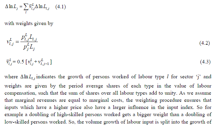 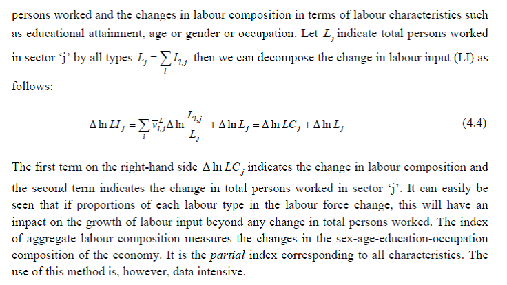 There is a second approach to the measurement of skill levels. The procedure is to use a simple index of educational attainment to adjust for skill differences. So the improvement in educational attainment is measured by incorporating average years of schooling as the proxy for skill levels. For example, an index of the form: L* = easL assumes that each year of schooling raises the average worker’s productivity by a constant percentage, ‘a’. Such studies have been carried out for different time periods and for a large number of countries around the world, typically finding a return to each additional year of education in the range of 7 to 12 per cent (BCV, 2007). Most of the recent indices of composition of labour input are based on the methodology of (JGF) Jorgenson, Gollop, and Fraumeni (1987) and use the Törnqvist translog index. However, this methodology requires a large volume of data. Using this methodology Sailaja (1988) obtained a similar index for output, labour and price in the case of Indian railways and Aggarwal (2004) estimated labour composition for the Indian manufacturing labour force. There are, however, a lot of disagreements on the use of this methodology in the Indian context, as it assumes the existence of perfectly competitive labour markets where wage rate is the indicator of a person’s marginal productivity. The analysts argue that the observed wage differences may reflect factors other than productivity differences, such as age or gender discrimination. Its use is also questioned because data for the large segment of Indian labour force- the self -employed is not available. Since the Indian labour market is still not very competitive and there are data weaknesses, the researchers in India have generally avoided applying the JGF methodology. For this reason, most Indian researchers have avoided to account for the differences in age and gender characteristics. However, to account for educational differences they have preferred to exercise either of the two choices - one to use Barrow and Lee (1993) methodology and presume a constant rate of return for education (BCV, 2007) or second is to use the limited information available on wages for few rounds and only for casual and regular employees (Sivasubramanian, 2004) to determine the weights of different types of persons. Bosworth and Collins (2008) assumed a constant annual return of 7 per cent for each additional year of education irrespective of the level of education. The problem with the assumption of uniform returns for each year is that it ignores all variations - across levels of education, over gender, over age groups, over industries, etc. and only includes education. It is thus not able to capture the impact of change in gender composition, age composition (a proxy for experience) and industry composition. The present study has adopted the middle path. While age and gender indices have been ignored because of lack of suitable data, labour composition indices in terms of educational differences have been developed using the JGF methodology. The data on employment is essentially derived from the unit level record data of National Sample Survey (NSS) which is made available by NSSO in the form of CD-ROMS for the five Quinquennial rounds beginning from 38th. We estimated the number of employed persons according to UPSS as follows:
For extrapolation backward to 1980-81 to 1982-83, the interpolation of the broad industrial classification of 32nd round and 38th round is used. So the estimates from 32nd round are mainly used as control numbers. For the construction of labour composition index, we require data on employment and earnings by education and by industry. We distinguish five types of educational categories for each of 27 industries. These are up to primary, primary, middle, secondary & higher secondary, and above higher secondary. Therefore the following additional steps have also been performed:
Once the above steps are taken to find out the educational distribution of all employed persons in all the six rounds and their corresponding wages, the computation of the labour education index is carried based on the JGF (1987) methodology with 1980-81 equal to 100. The education index is estimated for total persons working in 27 different industries in India for the 38th, 43rd, 50th, 55th, 61st, 66th and 68th rounds of NSSO with 1983 (38th round) equal to 100 so as to assess the temporal changes in labour skill. Since the series required is from 1980-81, we have extrapolated it backwards from 1983. The third phase of this project aims to perform some robustness checks and bring out policy implications from the employment trends. It also aims to update the labour input series to a more recent period. Appendix C: Definitions of Employment in NSSO Employment & Unemployment Surveys The surveys of NSSO on employment and unemployment (EUS) aim to measure the extent of ‘employment’ and ‘unemployment’ in quantitative terms disaggregated by various household and population characteristics following the three reference periods of (i) one year, (ii) one week, and (iii) each day of the week. Based on these three reference periods three different measures, termed as usual status, current weekly status, and the current daily status, are arrived at. While all these three approaches are used for collection of data on employment and unemployment in the quinquennial surveys, the first two approaches only are used for the purpose in the annual surveys. Usual principal status: In the NSS 27th round, the usual principal activity category of the persons was determined by considering the normal working pattern, i.e., the activity pursued by them over a long period in the past and which was likely to continue in the future. For the identification of the usual principal status of an individual based on the major time criterion, in NSS 27th, 32nd, 38th, 43rd rounds, a trichotomous classification of the population was followed, that is, a person was classified into one of the three broad groups ‘employed’, ‘unemployed’ and ‘out of labour force’ based on the major time criterion. From NSS 50th round onwards, the procedure was changed and the prescribed procedure was a two-stage dichotomous one which involved a classification into ‘labour force’ and ‘out of labour force’ in the first stage, and thereafter, the labour force into ‘employed’ and ‘unemployed’ in the second stage. Usual subsidiary status: In the usual status approach, besides principal status, information in respect of subsidiary economic status of an individual was collected in all employment and unemployment surveys. For deciding the subsidiary economic status of an individual, no minimum number of days of work during the last 365 days was mentioned prior to NSS 61st round. In NSS 61st round, a minimum of 30 days of work, among other things, during the last 365 days, was considered necessary for classification as usual subsidiary economic activity of an individual. Current weekly status: It is important to note at the beginning that in the EUS of NSSO, a person is considered as a worker if he/she has performed any economic activity at least for one hour on any day of the reference week and uses the priority criteria in assigning work activity status. This definition is consistent with the ILO convention and used by most of the countries in the world for their labour force surveys. In NSSO, prior to NSS 50th round and in all the annual surveys till NSS 59th round, data on employment and unemployment in the CWS approach was collected by putting a single-shot question ‘whether worked for at least one hour on any day during the last 7 days preceding the date of survey’. The information so collected was used to determine the CWS of the individuals. This procedure was criticised for being not able to identify the entire workforce, particularly among the females. It was then decided to derive the CWS of a person from the time disposition of the household members for the 7 days preceding the date of survey. The procedure was used for the first time in NSS 50th round. It is seen that the change in the method of determining the current weekly activity had resulted in increasing the WPR in current weekly status approach - more so for the females in both rural and urban areas than for males. The trend observed in NSS 50th round in respect of the WPR according to CWS suggested continuing with the procedure for data collection in CWS in NSS 55th and NSS 61st rounds. Current Daily Status: Current Daily Status (CDS) rates are used for studying intensity of work. These are computed on the basis of the information on employment and unemployment recorded for the 14 half days of the reference week. The employment status during the seven days is recorded in terms of half or full intensities. An hour or more but less than four hours is taken as half intensity and four hours or more is taken as full intensity. An advantage of this approach is that it is based on more complete information; it embodies the time utilisation and does not accord priority to labour force over outside the labour force or work over unemployment, except in marginal cases. A disadvantage is that it relates to person-days, not persons. Hence it has to be used with some caution. The Heckman model is formulated in terms of two equations: a selection equation – usually a Probit estimation (takes a value of 1 if a person is working, 0 otherwise) to explain the decision of whether to participate in the labour market and, a regression equation to explain days of actual labour market participation, observable only for those for whom the selection equation takes a value of 1. For the selection equation: zi*=wi γ + ui ; zi = 1 if zi*>0 and 0 otherwise Regression model: yi = xiβ + εi ; observed only if zi=1 It follows that standard regression techniques would yield biased estimates when ρ ≠ 0. Heckman provides consistent, asymptotically efficient estimates for all the parameters in such a model. In actual estimation, a likelihood ratio test of the independence of these equations testing for ρ = 0) with the corresponding chi-squared statistic is done. This technique helps us overcome the problem of not being able to observe the wage for those who are not employed in the reference period. The function has been used to estimate the earnings of casual and regular employees
Chapter 5: Capital Input Series at the Industry Level This chapter outlines the methodology employed to estimate capital services for the 27 industries in the India KLEMS database version 2015. Following an overview of the theoretical method developed by Jorgenson and Griliches (1967), and outlined in Jorgenson, Gollop and Fraumeni, (JGF, 1987), the chapter discusses the specific empirical approaches we follow to implement these methods within the constraints of data availability for Indian industries. For the measurement of capital services, we need capital stock estimates for detailed asset types and the shares of each of these assets in total capital remuneration. Using the Törnqvist approximation to the continuous Divisia index under the assumption of instantaneous adjustability of capital, aggregate capital services growth rate is derived as a weighted growth rate of individual capital assets, the weights being the compensation shares of each asset, i.e. 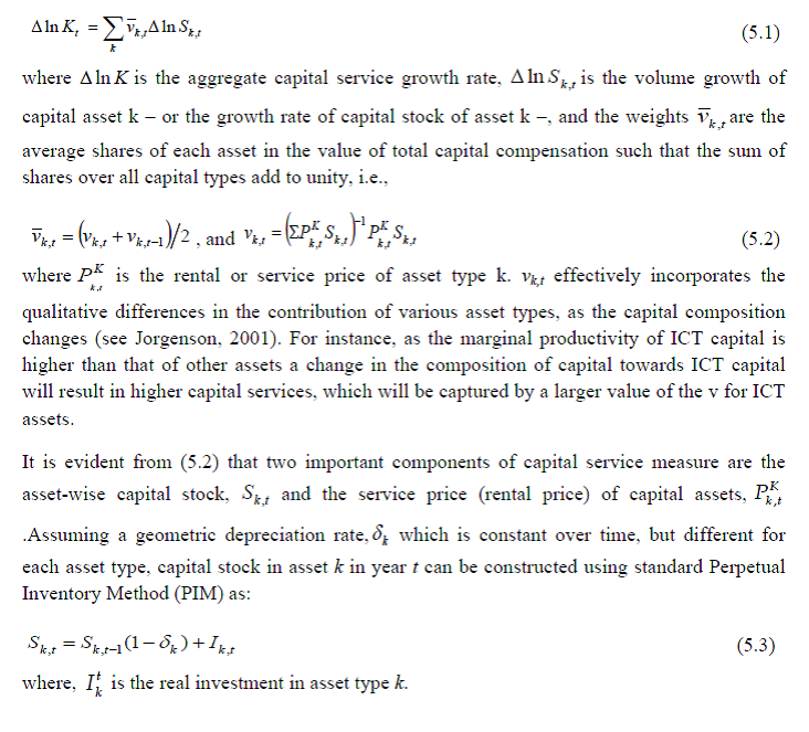 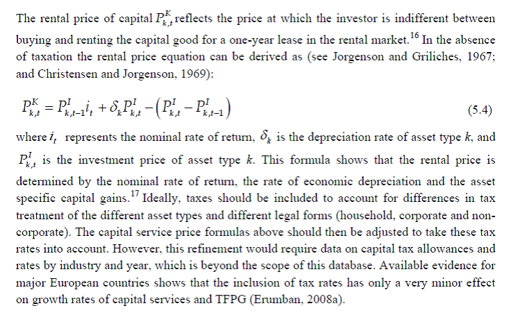 Since our measure of capital input takes account of asset heterogeneity, it was essential to obtain investment data by asset type. We distinguish between 3 different asset types – construction, transport equipment, machinery (includes ICT and non-ICT machinery).18 We exploit multiple sources of information for the construction of our database on capital services. This includes the National Accounts Statistics (NAS) that provide information on broad sectors of the economy, the Annual Survey of Industries (ASI) covering the organised manufacturing sector, the National Sample Survey Organizations (NSSO) rounds for unorganised manufacturing and Input-Output transaction tables. Even though we use multiple sources of data, our final estimates are fully consistent with the aggregate data obtained from the NAS. In addition, our approach to capital measurement is consistent with international practices such as the EU KLEMS19, which ensures the possibility of international comparisons. In what follows we discuss the various sources of data for asset-wise investment and the construction of the relevant variables, in detail. (a) Asset-wise investment for broad sectors of the economy Industry-level estimates of capital input require detailed asset-by-industry investment matrices. NAS provides information on aggregate capital formation by industry of use for 9 broad sectors, which, nevertheless, was not sufficient for our purpose. Therefore, we have collected more detailed data on assets and industries from the CSO.20 This is the data underlying the published aggregate gross fixed capital formation by the broad industry groups, separately for public and private sectors. For those sectors for which the investment matrices were not available from CSO, we gathered information from other sources (e.g. ASI for organised manufacturing and NSSO surveys for unorganised manufacturing) and benchmark it to the aggregate investment series from the National Accounts. Table 5.1 provides an overview of asset types available in NAS and their corresponding asset types used in our study.
Total investment in each asset category is calculated as the sum of private and public sector investment in each asset. Investment in transport equipment is not available separately for the private sector. We tried several approaches to impute the private sector transport equipment data. The first was to use the share of transport equipment in non-departmental enterprises. More specifically, we apply the non-departmental enterprise transport equipment to machinery & equipment (including transport equipment) ratio to machinery & equipment in private sector for each industry to obtain industry-wise transport equipment for the private sector. We take non-departmental enterprises only, rather than the entire public sector, as it may be more realistic as it consists of public sector companies and statutory corporations, excluding administrative sector. However, the sum of industry estimates generated by this approach was not consistent with the reported aggregate private sector transport equipment. Therefore, we take a second step here, which is to use the industry distribution from this series and apply it to the published total private sector transport equipment data. The estimated transport equipment is then subtracted from each industry’s total machinery & transport equipment data to obtain machinery in private sector as a residual. However, this approach generates many negative numbers in transport equipment in private sector, particularly in transport services. Therefore, we follow a third approach, which is what we finally use in the database. We first distribute the NAS total machinery in the private sector using the industry distribution of machinery and transport equipment. These estimates are then subtracted from each industry’s total machinery & transport equipment data to obtain the transport equipment investment in the private sector industries. (b) Asset-wise investment for non-NAS sectors NAS provides data only for 9 broad sectors, while we have 27 industries, which necessitated further splitting of some of the NAS sectors. This includes aggregate manufacturing (registered and unregistered separately) with 13 sub-sectors; other services into 4 sub-sectors; and real estate activities and business services into 2 sub-sectors. The manufacturing sector investment data was disaggregated into 13 sub-sectors at the 2-digit level of NIC 1998 using ASI and NSSO data, which will be discussed in detail subsequently. Investment series in the service sector has been split into sub-sectors using two alternative approaches–value added shares, and capital/labour ratio in the higher aggregate industry. However, the final data used are based on value added shares, as a sensitivity analysis did not show a significant difference between the two. In order to split the aggregate capital formation in organised manufacturing sector into 13 study sectors, we use the Annual Survey of Industries. However, the published data does not provide any asset-wise investment information; it consists of only the aggregate capital formation or the book value of fixed capital. Most studies in the past have measured gross investment as the difference between book value of the asset in period t and in period t-1 and add depreciation in period t to that. This approach has the deficiency of comparing two different samples reported in two different years, where the number of firms/factories might be different. In particular, while using this approach at the industry level, for detailed asset categories, it might generate massive negative investment. We follow an alternative approach, following ASI’s definition of gross fixed capital formation (GFCF). ASI defines GFCF as actual additions (newly purchased, second hand and own construction) minus deductions plus depreciation adjustment for discarded assets during the year. This approach is based on a single year’s sample and helps to avoid potential huge negative investment series and is also consistent with the published ASI GFCF series. The yearly detailed volumes beginning 1964-65 were used to derive the gross fixed capital formation by asset type directly. For the years 1964-1978, the relevant data are obtained from published detailed volumes. For the period, 1983-84 to 2004-05 ASI has generated detailed tables from Block C of ASI schedule that contain data on fixed assets. Data for missing years are interpolated using the changes in investment using book value method. Table 5.2 provides an overview of the asset categories available in ASI, and the relevant asset categories in our study to which they are attributed. Though ASI provides investment in land, for reasons of NAS consistency we exclude it from our database. Once the investment in each of these assets and industries are generated using ASI data, we apply this industry-asset distribution to the published aggregate NAS GFCF series for the organised manufacturing sector. It may also be noted that from 1960-61 to 1971-72, ASI data are for the census sector and from 1973-74 onwards they are for the factory sector. In order to make these two series comparable over years, we convert the data prior to 1972 to factory sector using the factory/census ratio in 1973. Thus, after these adjustments, we obtain investment data for 13 manufacturing sectors, by asset types, consistent with the NAS aggregates. The data required for creating the gross investment series for the 13 sectors of the unorganised manufacturing sector are obtained from various rounds of NSSO surveys on unorganised manufacturing. We use 4 rounds of NSSO surveys that cover the period 1989-2006. These are 45th round (1989-90), 51st round (1994-94) 56th round (2000-01) and 62nd round (2005-06). Unit level data has been aggregated to 13 industries using the appropriate concordance tables. NSSO provides net addition to owned assets during the reference year within the block of fixed assets, and we use this as a measure of our investment. Asset classification in NSSO has changed over various rounds, and therefore, we have tried to match these with our classification as shown in Table 5.3. The investment series arrived at for four rounds were interpolated to obtain the annual time series of unorganised gross fixed capital formation by asset type. As in the case of registered sector, once the investment by asset types across industries are constructed, the asset-industry distribution is applied to the published NAS aggregate GFCF in unregistered manufacturing to obtain NAS consistent GFCF by asset type and industries. (c) Investment Prices by Asset Types In order to compute asset-wise capital stock using PIM (equation 5.3) and rental price (equation 5.4), we require asset-wise investment price deflators. Since CSO has provided us with investment data by industries and assets both in current and constant prices, we could derive the price deflators with base 2004-2005. These deflators are directly used for all the three asset categories we have. (d) Initial Stock, Depreciation Rates and Rate of Return As is evident from equations 5.1 to 5.4, our estimates of capital input require time-series data on asset-wise capital stock. Capital stock has been constructed using perpetual inventory method (PIM), where the capital stock (S) is defined as a weighted sum of past investments with weights given by the relative efficiencies of capital goods at different ages, which requires data on current investment by asset types, investment prices by asset types and depreciation rate. Also, for the practical implementation of PIM to estimate asset-wise capital stock, we require an estimate of initial benchmark stock (see Erumban, 2008b for an in-depth discussion on this issue). NAS provides estimates of net capital stock since 1950 for all the broad sectors in its Statement 17: Net Fixed Capital Stock by industry of use. We take the NAS estimate of real net capital stock in 1950 (in 1999-2000 prices) as our benchmark stock for all non-manufacturing sectors, and for manufacturing sectors the same is taken for the year 1964.22 However, since the NAS estimate is available only for broad sectors and for aggregate capital, we use our industry-asset distribution of GFCF in order to create net fixed capital stock estimates by asset type for all the 27 industries. NAS also provides detailed tables on assumed life of assets used for computing capital stock, for private units, administrative units as well as departmental and non-departmental units by asset types.23 We use these estimates of lifetime to derive appropriate depreciation rates for non-ICT assets, using a double declining balance rate. We assume 80 years of lifetime for buildings, 20 years for transport equipment, and 25 years for machinery and equipment. The final depreciation rates used in the study are given in Table 5.4 by asset type. Subsequently, we build our capital stock series by asset types for all the 27 industries using our GFCF series from 1950 (1964) onwards for the non-manufacturing (manufacturing) sectors. Our measure of capital input is arrived using equation (5.1), for which we also require estimates of rental prices (see equation 5.4). Assuming that the flow of capital services is proportional to the capital stock at the individual asset level, aggregate capital flows can be obtained using a translog quantity index by weighting growth in the stock of each asset by the average shares of each asset in the value of capital compensation, as in (5.1). The rate of return (i) in equation (5.4) represents the opportunity cost of capital and can be measured either as internal (or ex-post) rate of return or as an external (ex ante) rate of return.24 This issue will be addressed in the further revisions of the data. The present version of the database uses an external rate of return, proxied by average of return on government securities and prime lending rate obtained from the Reserve Bank of India25. Therefore, we use a real rate, which is net of capital gain. Hence, the capital gain component in equation (5.4) is excluded while estimating rental price using external rate of return, obtaining 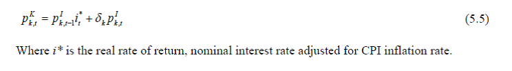 Chapter 6: Intermediate Input Series at the Industry Level In this section, we describe the basic approach we have used to derive the volume series of Intermediate Inputs namely – Energy input (E), Material input (M) and Services input (S). This breakdown of intermediate inputs can be used for extending the growth accounting exercises, but also convey interesting information about changing pattern in intermediate consumption (see e.g. JHS 2005, Chapter 4) The methodology for measuring industry output, intermediate inputs and value added was developed by Jorgenson, Gallop and Fraumeni (1987) and extended by Jorgenson (1990 a). The cornerstone of this approach is a time series of input-output (IO) tables, which gives the flows of all commodities in the economy, as well as payments to primary factors. Every commodity is accounted for, whether produced by a domestic source or imported, and every use is noted, whether purchased by an industry or by a final demand element. All payments to factors of production i.e., labour and capital are accounted for so that all income elements of GDP are included. The methodology of constructing time series on energy, material and services inputs for the European economy has been elucidated in Timmer et al. (2010, Chapter 3). Following a similar approach as explained in Jorgenson et al. (2005, Chapter 4) and Timmer et al. (2010, Chapter 3), the time series on intermediate inputs for the India KLEMS project have been constructed. Definition of EMS: As in EU KLEMS, this study identifies three main categories of intermediate inputs. They are classified as follows:
Intermediate inputs are broken down into energy, material and services, based on input-output transaction tables using a standard NIC product classification. The following five energy types (and products) have been classified as the Energy input.
The following fourteen input items have been classified as the Service input
All other intermediate inputs barring the above-mentioned nineteen inputs are classified as material input. The key building block for constructing Time Series on intermediate inputs at current prices, as explained in Jorgenson et al. (2005, Chapter 4), is the input-output transaction tables, that is, the inter-industry transaction tables that provide a description of which industries produce each product and which industries use them. The IOTT gives the inter-industry transactions in value terms at factor cost presented in the form of commodity x industry matrix where the columns represent the industries and the rows as group of commodities, which are the principal products of the corresponding industries. Each row of the matrix shows in the relevant columns, the deliveries of the total output of the commodities to the different industries for intermediate consumption and final use. The entries read down industry columns give the commodity inputs of raw-materials and services, which are used to produce outputs of particular industries. The column entries at the bottom of the table give net indirect taxes (NIT) (indirect taxes – subsidies) on the inputs and the primary inputs (income from use of labour and capital), i.e., Gross Value Added (GVA). As the IOTT is in the form of commodity x industry matrix, the row totals do not tally with the column totals. The difference between each column and the corresponding row totals is due to the inclusion of the secondary products, which appear particularly in the case of manufacturing industries. This is so because by-products are also manufactured by industries in addition to their main products. Thus, while determining the entries in the rows, a by-product of an industry is transferred to the sector (commodity row), whose principal product is the same as the by-product under reference. The columns, however, show the total of principal products and by-products of each industry. All the entries in the IOTT are at factor cost, i.e. excluding trade and transport charges and NIT. The Input Flow Matrix at factor cost, published by CSO, for 1978 is a 60 x 60 matrix. The absorption matrices for 1983, 1989, 1993 and 1998 have 115 sectors. However, a detailed 130 sector absorption (commodity x industry) matrix for the Indian economy has been published from 2003-04 onwards. The scheme of sector classification adopted in IOTT 2007-08 and IOTT 2003-04 viz., IOTT 1983-84, IOTT 1989-90, IOTT 1993-94 and 1998-99 has undergone significant change with the disaggregation of some of the sectors, which have become significant in the early 2000s.
The methodology for computation of intermediate input series for 27 Industries from 1980-2011 at current and constant prices is explained in steps. Step 1: Concordance is done between IOTT and study industries
Step 2: Obtaining estimates for Material, Energy and Service Inputs for 27 Industries, in benchmark years In IOTT, no intermediate input is being used in industry 24 – ‘Public Administration’. Consequently, the intermediate input series is being estimated for only 27 industries from 1980 to 2011. The 60/115/130 commodity inputs going into the production process of output for 27 industries are aggregated into
Thus, for each of the benchmark years, estimates are obtained for Material, Energy and Service Inputs that has been used to produce Gross output in the 27 different India KLEMS Industries. Step 3: Projecting a time series (1980 to 2011) of proportions of Material, Energy and Service Inputs in Total Intermediate Inputs for each of the 27 industries
Step 4: Consistency with NAS The projection of intermediate input vector, using IOTT in Step 3 needs to be consistent with the estimated output from NAS.
1. For Benchmark years: Ratio of total intermediate inputs from NAS to that from IOTT is adjusted proportionately to the absolute value of Energy /Material /Service Inputs obtained from IOTT. 2. For Intervening Years: The interpolated proportions of energy, material and services inputs obtained from IOTT, are applied directly to the total intermediate inputs from NAS to get share of each inputs. Two examples have been given below for the construction sector:
In the examples above, we can see that the total value of intermediate input exactly matches the gap between the gross value of output and gross value added. Similar adjustments have been made to construct the input series for all the other 27 study industries from 1980-2011. For every benchmark year where IOTT is available, adjustment ‘A’ has been done. For every non-benchmark year, where IOTT is not available and an intermediate input vector has been projected, adjustment ‘B’ has been done to generate the comprehensive time series of intermediate inputs consistent with the official National Accounts. Steps 1-4: This gives a Time Series of Material, Energy and Service Inputs for 27 Study Industries from 1980 to 2011 at current prices. Steps 5 and 6 below, explain the methodology for computation of intermediate input series for 27 study Industries from 1980-2011 at constant price. The approach followed here is to first form the aggregates of materials, energy and services at current price for each study industry from the benchmark Input-Output tables and then develop deflators of materials, energy and service inputs for each of the 27 study industries separately. Step 5: Constructing Deflators of Materials, Energy and Service Inputs for 27 Study Industries separately
Step 6: Computing Time Series on Intermediate Input for 27 study Industries from 1980-2011, Constant prices
Thus, we have a time series of material, energy and service inputs for 27 study Industries at constant prices. Aggregation: The report identifies six broad sectors of Total Economy. They are Agriculture; Mining and Quarrying; Manufacturing; Electricity, Gas and Water Supply; Construction and Services. For aggregation of industries, we use Tornqvist quantity index, which is a discrete time approximation to a Divisia index. This aggregation uses annual moving weights based on averages of adjacent points in time. The advantage of Tornqvist index is two-fold. First, it belongs to the preferred class of superlative indices (Diewert 1976). It exactly replicates a translog model which is flexible, that is, a model where aggregate is a linear and quadratic function of the components and time. Secondly, Tornqvist index is relatively easy to implement. Firstly, Input-Output transaction tables are generally available on a five year interval period and this necessitates interpolation and assumption of constant shares in some cases to construct the entire time series of EMS from 1980 to 2011. Secondly, unlike studies using detailed survey data, we have to assume that all buyers pay the same price for each commodity because there is no information about price divergences. Thirdly, the estimated time series of intermediate inputs at constant prices will not be consistent with the intermediate input of NAS at constant price i.e., the deflated value of intermediate input cannot match the gap between value added and gross output at constant price from NAS. This is because NAS uses a single deflation method to estimate Gross Value Added and Gross Value of Output at constant prices. ‘However, only for one sector – Agriculture, the Gross Output and Gross Value Added, estimated by NAS is double deflated. Therefore, only for the Agriculture sector, the deflated value of intermediate input will exactly match the gap between value added and gross output at constant prices. Fourthly, there has been some confusion in the literature on the price concept to be used for intermediate inputs. It is generally acknowledged that the intermediate input weights should be measured from the user’s point of view, i.e., reflect the marginal cost paid by the user. Most studies maintain that purchaser’s price should be used. These prices include net taxes on commodities paid by the user and include margins on trade and transportation (see, for example, OECD 2001). However, when trade and transportation services are included as separate intermediate inputs, margins paid on other products should also be allocated to these services. Ideally, a distinction should be made between the intermediate product valued at purchaser’s price minus margins and the trade and transportation services valued at margins. This is the approach taken in Jorgenson, Gollop and Fraumeni (1987) and in Jorgenson et al. (2005). However, Timmer et al. (2010, Chapter 3) explains that for the EU KLEMS database, intermediate inputs have been valued at purchaser’s price owing to unavailability of necessary data. Because of the use of purchaser’s price concept the shares of services in intermediate inputs do not include trade and transportation margins. Similarly, in practice for the database, the time series of Intermediate Input constructed is at purchaser’s price i.e. it implicitly takes into account the net indirect taxes. The distribution of this net indirect tax between material, energy and services has not been possible because of unavailability of a time series of tax matrix from 1980 to 2011. Chapter 7: Factor Income Share Series at the Industry Level The distribution of income between capital, labour and intermediate inputs, is an important element in growth accounting because income shares, under conditions of competitive markets, can be used to measure the contributions each factor makes towards output growth. 7.1 Methodology for Measuring Labour Income Share Series Under the assumption of constant returns to scale with two factors of production i.e., labour and capital, the sum of the labour income share and capital income share is 1. The labour income share is defined as the ratio of labour income to GVA. Capital income share is accordingly obtained as one minus labour income share. There are no published data on factor income shares in Indian economy at a detailed disaggregate level. National Accounts Statistics (NAS) of the CSO publishes the Net Domestic Product (NDP) series comprising of compensation of employees (CE), operating surplus (OS) and mixed income (MI) for the NAS industries. The income of the self-employed persons, i.e. MI is not separated into the labour component and capital component of the income. Therefore, to compute the labour income share out of value added, one has to take the sum of the compensation of employees and that part of the MI which are wages for labour. The computation of labour income share for the 27 study industries involves two steps. First, estimates of CE, OS and MI have to be obtained for each of the 27 study industries from the NAS data which are available only for the NAS sectors (see Table 7.1). Second, the estimate of MI has to be split into labour income and capital income for each industry for each year (except for those industries for which the reported MI is zero, for instance, public administration). Basic data sources used for the computation of labour income share are NAS, ASI and unit level data of survey of unorganised manufacturing enterprises. These data sources are used to obtain estimates of CE, OS and MI for each of the 27 study industries. For splitting the labour and non-labour components out of the MI of self-employed, the unit level data of NSS employment-unemployment surveys are used along with the estimates of CE, OS and MI basically obtained from the NAS. a) Construction of Labour Income Share Series in Gross Value Added The estimation of labour income share for the 27 study industries has been done in two steps, as discussed below. Step 1: Estimation of CE, OS and MI for the 27 study Industries For some industries under study, for instance (i) Agriculture, forestry & logging and fishing, (ii) Mining & quarrying, (iii) Electricity, gas and water supply, and (iv) Construction, the required data are readily available from NAS. For others, the estimates available in NAS have to be distributed across the study industries. In certain cases, the estimates of CE, OS and MI for a particular NAS sector have been distributed across constituent study industries proportionately in accordance with the gross value added in those industries. Estimate of factor incomes for ‘other services’ in NAS, for instance, has been split into estimates for (i) Education, (ii) Health and Social Work, and (iii) Other Community, Social and Personal Services including Renting of machinery and business services, and Private Household with Employed Persons. NAS provides estimates of factor incomes for registered manufacturing and unregistered manufacturing, but not for individual manufacturing industries. The NAS estimates of factor incomes for registered manufacturing have to be split into various manufacturing industries considered in the study (13 in number) using ASI data. The reported CE in NAS for registered manufacturing has been distributed into those 13 industries in proportion to the reported ASI data on emoluments for various industries. In a similar way, using ASI data, the estimate of OS for registered manufacturing has been distributed. Emoluments are subtracted from gross value added for various industries yielding capital income. The share of different industries in aggregate capital income of organised manufacturing indicated by the ASI data is used to split the estimate of OS for registered manufacturing reported in the NAS. The methodology applied for unregistered manufacturing is similar. The published results and unit level data of survey of unorganised manufacturing industries have been used for this purpose. The estimates of wage payments (to hired workers) in different industries have been used to split (proportionately) the estimate of CE in the NAS for aggregate unregistered manufacturing. The estimated wage payment is subtracted from the estimated value added to obtain an estimate of capital income and mixed income of the self-employed in various unorganised manufacturing industries. The estimate of MI provided in NAS for unregistered manufacturing has then been proportionately distributed across industries using the estimate of capital income and mixed income of the self-employed in various industries that could be formed on the basis of published results and unit level data of survey of unorganised manufacturing industries. Unlike the ASI data for organised manufacturing, the data for unorganised manufacturing enterprises are available for only select years. The proportions mentioned above could, therefore, be computed only for those select years (data for five rounds have been used; these are for the 45th round (1989-90), 51st round (1994-95), 56th round (2000-01), 62nd round (2005-06) and 67th round (2010-11)). It has accordingly been necessary to resort to interpolation/ extrapolation to obtain the relevant proportions for other years. Step 2: Splitting of MI into Labour Income and Capital Income As explained above, the income share of labour is computed as: 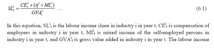  The derivation of the GVA series for different industries has been briefly explained in Chapter 2. The derivation of CE and MI series has been explained in step I above. Therefore, only the estimation method of ƞ needs to be described. The estimation of ƞ has been done with the help of NSS survey-based estimates of employment of different categories of workers (number of persons and days of work) and wage rates (which has been described briefly in Chapter 4) coupled with estimates of MI, basically obtained from the NAS. Two approaches have been taken to get an estimate of ƞ, and the labour income share series for different industries finally adopted in the study makes use of an average of the estimates of ƞ obtained by the two approaches. In the first approach, an estimate of labour income of self-employed workers has been made for each study industry for five years, 1983-84, 1987-88, 1993-94, 1999-00, 2004-05, 2009-10 and 2011-12 on the basis of the estimated number of self-employed, wage rate of self-employed and the number of days of work per week. The industry-wise estimates of number of self-employed, wage rate of self-employed and the number of days of work per week has been made from unit records of NSS employment-unemployment surveys (major rounds), as explained in Chapter 4 above. The estimates of the number of self-employed, wage rate of self-employed and the number of days of work per week provide an estimate of the annual labour income of self-employed workers which is divided by the mixed income of self-employed (derived from NAS) to get an estimate of ƞ. For five industries, the ratio in question has been computed and applied. For the other 22 industries, the ratio in question has been computed after clubbing the industries into 11 industry groups.26 In the latter case, a common ratio computed for a group of industries has then been applied to constituent industries. The list of industries or industry groups for which ƞ has been estimated is given in table 7.2. In the second approach, the NSS data are used to compute the following ratio: the ratio of labour income of self-employed workers to the labour income of regular and casual workers. Let this be denoted by θ. Then, the estimate of CE provided in the NAS is multiplied by θ to obtain an estimate of the labour income component out of the MI reported in the NAS. The labour component of MI divided by total MI gives an estimate of ƞ. In case the estimated labour component of MI exceeds the estimate of MI, the estimate of ƞ has been taken as unity. Examining the estimates obtained by the first approach, it was found that the estimated labour income share out of mixed income varied significantly among the estimates for the seven years for which the ratio in question has been estimated. The estimates of ƞ obtained by the second approach has the problem that in a number of cases, the estimated labour component of MI exceeds the estimate of MI given in the NAS, and therefore ƞ is taken as one. The method finally adopted is as follows: (a) The average value of ƞ has been computed for each industry or industry group by taking the estimates for the years 1983-84, 1987-88, 1993-94, 1999-00, 2004-05, 2009-10 and 2011-12. This has been done separately for the estimates based on approach-1 and those based on approach-2. (b) The estimates of ƞ obtained for each industry or industry group by the two approaches have then been averaged. (c) Having obtained an estimate of ƞ, equation 6.1 given above has been applied to compute the labour income share. b) Construction of Factor Income Share Series in Gross Output The income share of labour, capital and intermediate inputs in Gross output has been computed using the following steps:
The splitting of unorganised sector factor incomes into individual industries has been done using unorganised sector survey results. The proportions computed for 1983-84 has been applied for the period 1980-81 to 1983-84. While there were surveys of unorganised manufacturing enterprises in 1978-79 and 1984-85, the survey results have not been used for estimation of factor incomes in different industries of the unorganised manufacturing sector. An attempt will be made to use survey data for the years 1978-79 and 1984-85 rather than applying the proportions computed for 1989-90 to factor income data for earlier years. The present study provides estimates of income shares for manufacturing and its sub-branches. An attempt will be made in the third phase of the study to split manufacturing sector into organised manufacturing and unorganised manufacturing segments. The output and inputs series will be constructed separately for organised and unorganised manufacturing sectors. However, given the employment potential and sizable presence of the unorganised segment in many of the manufacturing industries, it would be worthwhile in Indian context to examine separately the productivity performances of the organised and unorganised components of Indian manufacturing. Thus, in the third phase of this project, the labour income series will have to be computed for the organised and unorganised sectors manufacturing separately. Chapter 8: Growth Accounting Methodology This chapter deals with the methodology of measurement of total factor productivity (TFP) growth for individual industries in the KLEMS framework and the aggregation from industry level productivity measures to measures for broad sectors and the economy as a whole. The methodology of analysis of sources of gross output growth at the individual industry level and sources of GVA (Gross Value Added) or GDP growth at the broad sector level and the economy level will also be presented in this chapter. 8.1 Methodology for Measuring Productivity Growth at the Industry level The production function Our measurement of TFP growth for different industries of the Indian economy is based on a gross output production function for each industry j: Y = f (L (L1,…Ln), K (K1…Km), E (E1….Es), M (M1 …Mu), S (S1 … Sv ), T) (8.1) Y is industry gross output, L is labour input, K is capital input and E, M and S are intermediate inputs-namely energy, material and services and T is an indicator of technology for industry j. All variables are indexed by time (t subscript is suppressed). There are several things to note about the production function- (1) all variables are aggregates of many components that have been discussed in the earlier report/ chapters; (2) we assume that the industry production function is separable in these aggregates; (3) time (indicator of technology) enters the production function symmetrically and directly with inputs. An important feature of the gross output approach is the explicit role of intermediate inputs. In our study, we have considered three intermediate inputs - energy, material and services and this is important as we may find that intermediate inputs are the primary component of some industries outputs.27 Failure to quantify intermediate inputs leads us to miss both the role of key industries that produce intermediate inputs and the importance of intermediate inputs for the industries that use them. In order to estimate the production function at constant prices, the industry level price data is used for output, capital, labour and intermediate inputs, e.g., PYj; PLj, PKj; PEj, PMj, PSj. We assume that all industries face the same input prices. The industry price of an input varies across industries due to compositional effects as industries expend different shares of their investment on each type of asset. The same is true for all inputs. 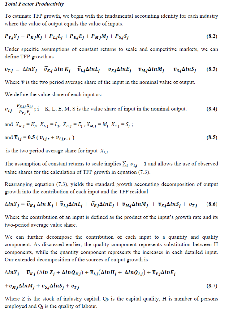 8.2 Methodology for Aggregation across Industries In the analysis presented in the above section, gross value of output (GVO) is taken as the measure of output of an industry and TFP growth was estimated using the gross output function framework in which capital, labour, material, energy and services are taken as five inputs (in the case of agriculture, land was included among inputs). The Tornqvist index is applied to estimate TFP growth for each year during 1980-81 to 2011-12, which yielded an index of TFP for each industry for that period, permitting estimation of trend growth rate in TFP for the period under study (1980-81 to 2011-12). The method of estimation of TFP growth for individual industries described in section 7.1 cannot be readily applied to a higher level of aggregation. The main problem is that gross value of output cannot be added across industries to generate a measure of output at a higher level of aggregation, say for the economy or of any of the broad sectors. It becomes necessary, therefore, to consider appropriate methods of aggregation across industries consistent with the gross output function specification at the individual industry level. It is needless to say that one has to use the concept of value added to define an appropriate measure of output at the economy or broad sector level, but even here there are important issues of aggregation, i.e., how value added in different industries should be combined. A very useful discussion of the issues involved is found in Jorgenson et al. (2005). There are three approaches to estimating TFP growth at an aggregate level. This is discussed in detail in Jorgenson et al. (2005). The first approach is called aggregate production function approach. This approach assumes the existence of an aggregate production function (say, at the level of the economy or at the level of manufacturing or services sector). An essential condition is that the production function be separable in primary inputs. Let the production function for a particular industry be defined as: Y =f (X, K, L, T), (8.8) where Y denotes gross output, X intermediate input (in turn a combination of material, energy and services), K capital input, L labour input and T time (representing technology). Then, the concept of value added requires the existence of a value added function which in turn requires that the above production function be separable in K, L and T, i.e., the production function should take the following form: Y =g (X, V (K, L, T)). (8.9) In this equation, V (.) is the value added function. V denotes value added. Besides the condition of separability of the production function described above, a number of highly restrictive assumptions have to be made for the aggregate production function approach. These include: (a) the value added function is the same across all industries up to a scalar multiple, (b) the functions that aggregate heterogeneous types of labour and capital must be identical in all industries, and (c) each specific type of capital and labour receives the same price in all industries. With these assumptions made, real value added at the aggregate level becomes a simple addition of real value added in individual industries. In notation, 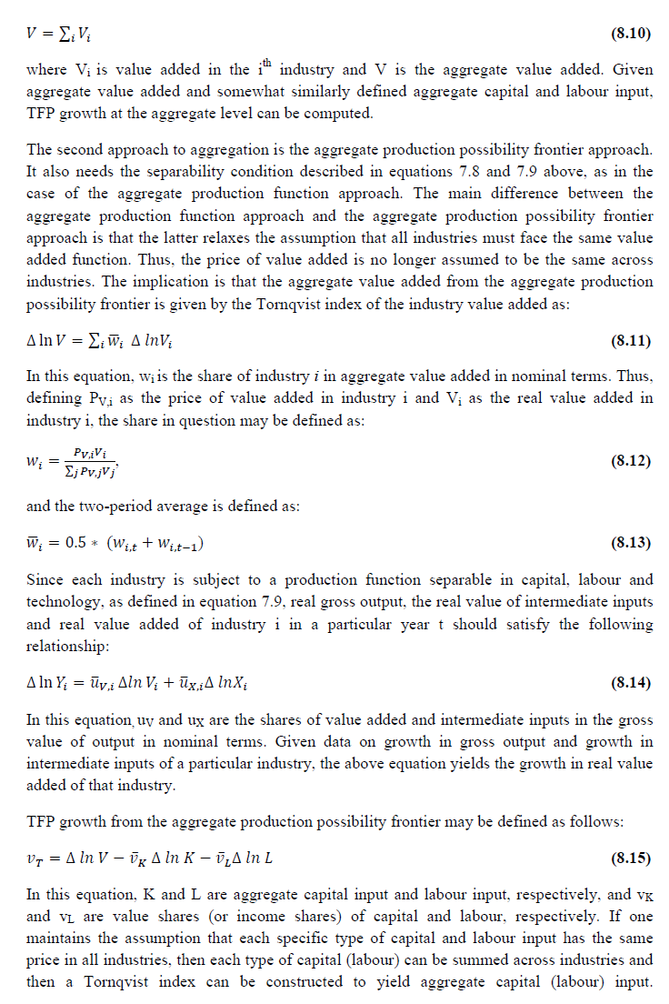 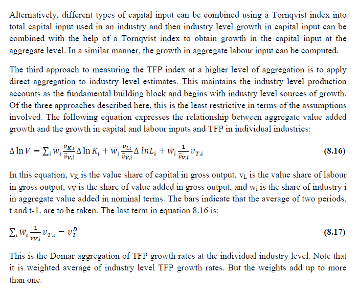 The data constructed for gross value added and gross output, labour input, capital inputs, intermediate inputs and factor income shares (Chapters 2, 3, 4, 5, 6 and 7 respectively), are used to estimate TFPG during the period 1980 to 2011. Labour input is measured using total person worked (see, Chapter 4 for the detailed discussion). The series on investment in capital services (including ICT) are taken from Chapter 5. Bibliography Aggarwal, Suresh Chand (2004), “Labour Quality in Indian Manufacturing: A State Level Analysis”, Economic and Political Weekly, Vol. 39(50), pp.5335‐44. Bhalla, Surjit S. and Tirthatanmoy Das (2005), “Pre‐ and Post‐Reform India: A Revised Look at Employment”, Wages and Inequality, India Policy Forum, Vol. 2, NCAER, New Delhi. Bosworth B., Collins S. and Virmani A. (2007), “Sources of Growth in Indian Economy”, NBER Working Paper No. 12901. Bosworth, Barry and Susan M. Collins (2008), “Accounting for Growth: Comparing China and India”, Journal of Economic Perspectives, American Economic Association, Winter, 22(1): 45‐66. Christensen, L.R. and Jorgenson D.W. (1969), “The Measurement of US Real Capital Input, 1929‐x”, Review of Income and Wealth, 15, 293‐320. CSO (2007), “National Accounts Statistics: Sources and Methods”, available at http://mospi.nic.in/ Central Statistical Organization: Population of India, different years. Diewert, W.E. (1976), “Exact and Superlative Index Numbers”, Journal of Econometrics, 4, 115‐145. Diewert, E (1980), Aggregation Problems in the Measurement of Capital, in Usher, D (eds.), The Measurement of Capital, Chicago, The University of Chicago Press. Erumban, A, A (2008a), “Rental Prices, Rates of Return, Capital Aggregation and Productivity: Evidence from EU and US”, CESifo Economic Studies, 3 (54), 499‐533. Erumban, A, A (2008b), Measurement and Analysis of Capital, Productivity and Economic Growth, SOM theses series, University of Groningen (available http://irs.ub.rug.nl/ppn/315102683). Jorgenson, D.W and Z. Griliches (1967), “The Explanation of Productivity Change”, Review of Economic Studies, 34, 249‐283. Jorgenson, D. W. et al. (1987), Productivity and US Economic Growth, Harvard University Press, Cambridge Mass. Jorgenson, D and K Vu (2005), “Information Technology and the World Economy”, Scandinavian Journal of Economics 107(4), 631-650, 2005. Jorgenson D.W. and Stiroh K.J. (2000), “Raising the Speed Limit: U.S. Economic Growth in the Information Age”, Brookings Papers on Economic Activity, (1), 125‐211. Jorgenson, D. W., Ho, M. S. and Stiroh, K. J. (2005), “Information Technology and the American Growth Resurgence”, MIT Press, Cambridge. OECD (2001): OECD Productivity Manual, Paris. O’Mahony, M. and M.P. Timmer (2009), “Output, Input and Productivity Measures at the Industry Level: The EU India KLEMS database”, Economic Journal, 119(538), pp. F374‐ F403. Rangarajan C. (2009), India Monetary Policy, Financial Stability and Other Essays, Academic Foundation, New Delhi. Sailaja, M. (1988), Productivity in the Service Sector: The Case of Indian Railways, 1950‐ 51 to 1985‐86, unpublished Ph.D. thesis, Delhi School of Economics, Delhi. Sivasubramanian S. (2004), The Sources of Economic Growth in India: 1950‐51 to 1999‐ 2000, New Delhi: Oxford University Press. Srinivasan, T. N. (2008), “Employment and Unemployment since the Early 1970’s”, India Development Report, OUP, Mumbai. Sundaram, K. (2007), “Employment and Poverty in India, 2000‐2005”, Economic and Political Weekly, Vol. XLII (30), pp. 3121‐31. Sundaram, K (2009), “Measurement of Employment and Unemployment in India: some issues”, Working Paper No. 174, Centre for Development Economics, Department of Economics, Delhi School of Economics, Delhi. Timmer, M.P, Mahony, M. and van Ark, B. (2007), The EU KLEMS Growth and Productivity Accounts: An Overview, Mimeo University of Groningen & University of Birmingham. Timmer, Marcel P.; Robert Inklaar; Mary O’Mahony and Bart van Ark (2010), Economic Growth in Europe: A Comparative Industry Perspective, Cambridge: Cambridge University Press. Visaria, P (1996), “Structure of Indian Workforce, 1961‐1994”, Indian Journal of Labour Economics, New Delhi, pp.725‐739. 1 Timmer, M.P, Mahony, M. and van Ark, B. (2007). The EU KLEMS growth and productivity accounts: an overview. Mimeo University of Groningen & University of Birmingham, 2 Readers can refer to India KLEMS Data Manual Version 2013 for the data set released by RBI on its website in June 2014. 3 From both aggregated 9 NAS sectors Gross Domestic Product by economic activity statement along with the disaggregated statements of these 9 NAS sectors. 4 It uses NAS Series 2004-05 for more recent years. 5 The principle components of manufacturing n.e.c are manufacturing of jewellery and related articles, manufacture of musical instruments, manufacture of sports goods, manufacture of games and toys and other manufacturing. 6 See Himanshu (2011) for a discussion on many issues associated with the NSSO employment surveys. 7 The coverage and the sample size of thin rounds is different from major rounds. 8 Problems in using UPSS are: The UPSS seeks to place as many persons as possible under the category of employed by assigning priority to work; there is no single long-term activity status for many as they move between statuses over a long period of one year, and Usual status requires a recall over a whole year of what the person did, which is not easy for those who take whatever work opportunities they can find over the year or have prolonged spells out of the labour force. 9 In EU-KLEMS changes in labour composition has been measured by including employment class, gender, age and education (Timmer, op cit; p64) and only 3 categories of education defined as high skilled, medium skilled and low skilled have been taken. This concept of labour composition is referred as ‘labour quality’ by Jorgenson. It is recognised (Timmer; op cit; p84) that the categorisation may lead to biases in the aggregate composition adjustment if employment trends and wage share differ within categories. These education categories generally correspond to- up to Primary education, above Primary to Hr. Secondary education and above Hr Sec or College education. Due to data limitations in India we have measured changes in labour composition only by changes in education profile of labour; hence named it labour education index. Therefore it became necessary to have a more detailed classification of education to capture the changes in skill composition of labour in India. For comparison, we estimated the changes in labour composition based on three education categories also and found that for the total economy the annual trend growth in labour education index is 1.16 per cent as compared to 1.25 per cent based on five education categories. 10 This procedure has been advocated by NSSO itself and has been consistently adopted by almost all researchers. 11 A very lucid description of the same is given by Sivasubramanian (2004). 12 Aggregate input is measured as a translog index of its individual components. Then the corresponding index is a Törnqvist volume index (see Jorgenson, Gollop and Fraumeni 1987). For all aggregation of quantities we use the Törnqvist quantity index, which is a discrete time approximation to a Divisia index. This aggregation approach uses annual moving weights based on averages of adjacent points in time. The advantage of the Törnqvist index is that it belongs to the preferred class of superlative indices (Diewert 1976). Moreover, it exactly replicates a translog model which is highly flexible, that is, a model where the aggregate is a linear and quadratic function of the components and time. 13 Although census population is available only decennially, we used the interpolated population figures for the mid-year survey periods [Visaria, (1996) for 1977-78 (Jan) and 1987-88 (Jan); Sundaram, (2007) for 1983 (July), 1993-94 (Jan), 1999-00 (Jan) and 2004-05 (Jan)] and from NSSO (2010) for Jan 2010. 14 In EU KLEMS (Timmer, op cit; p 67) it is assumed that the earnings is equal to the earnings of ‘regular' employees. 15 The details of the function can be obtained from the Stata software and from Appendix. 16 Asset prices are used in the aggregation of capital stock. However, it is the price of the capital service that must be used in aggregating capital services (see Jorgenson and Griliches, 1967; Diewert, 1980) as it is the services delivered by capital goods that are used in the production process,. Jorgenson and Griliches (1967) have shown that these two prices are related; the asset prices are the discounted value of all future capital services. They are not proportional though, as there are differences in replacement rates and capital gains among different capital assets. 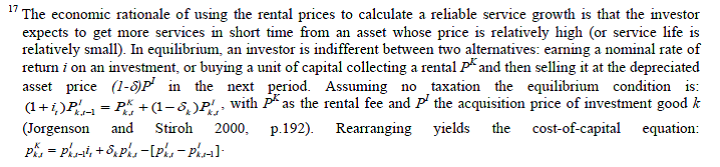 18 This version of the database does not make a distinction between ICT and non-ICT assets, as the industry level data on ICT assets are weak. An attempt to estimate aggregate economy level ICT capital can be found in Erumban and Das (2015). 19 See O’ Mahony and Timmer (2009) for a description of EU KLEMS database 20 This data is not publicly available. However, CSO has been kind to compile this data for the India-KLEMS project. 21 In some years transport equipment was provided as part of the machinery and equipment, categorized as ‘tools, transport equipment and other fixed assets’. In such cases, we use transport/tools, transport and other fixed asset ratio in the nearest year to separate transport equipment. 22 This choice is driven by the fact that the first year of availability of ASI data is 1964-65. 23 National Accounts Statistics-Sources and Methods, Chapter 26, CSO (2007) 24 We do not intend to delve into the controversies over the use of internal vs. external rate of return in the context of productivity measurement. Rather, given that this is the first version of our data, we use the external rate and in a later stage, we will also use internal rates. See Erumban (2008a and b) for a discussion on these issues. 25 Reserve Bank of India, Handbook of Indian Statistics, Annual volumes. 26 The estimation is done at group level rather than individual industries on the consideration that the group level estimates will be more reliable. 27 Consider, the semi-conductor (SC) industry, which is a key input to the computer hardware industry. Much of the output is invisible at the aggregate level because semi-conductor products are intermediate inputs to other industries rather than deliverables to final demand- consumption and investment goods. Moreover, SC plays a role in the improvements in quality and performance of other products like-computers, communication equipments and scientific instruments. Failure to account for them leads us to miss the role of key industries that produce intermediate inputs and importance of intermediate inputs for the industries that use them (Jorgenson, Ho and Stiroh (2005), Productivity, volume 3). |
||||||||||||||||||||||||||||||||||||||||||||||||||||||||||||||||||||||||||||||||||||||||||||||||||||||||||||||
Measuring Productivity at the Industry Level - The India KLEMS Database
|
AUTHORS Deb Kusum Das Abdul Azeez Erumban Suresh Aggarwal Pilu Chandra Das NEW ADDITIONS TO DATA MANUAL 2016 (Version 3) The dataset includes measures of Gross Value Added (GVA), Gross Value of Output (GVO), Labour (L), Capital Stock (K), Energy (E), Material (M), Services (S), Labour Quality (LQ), Capital Composition (KQ) and Total Factor Productivity (TFP) at the industry level from 1980-81 to 2014-15. Gross Value Added: Up to 2011-12, estimates of GVA for all industries are directly obtained from Back Series 2011 and NAS 2014. Onwards 2012-13, GVA series are extended using annual growth rate estimated from NAS 2016 (this has been done because of the introduction of the new National Accounts series with base 2011-12). NAS provide separate estimates of GVA for registered and unregistered manufacturing. However, onwards 2011-12 NAS disaggregated the manufacturing sector in corporate sector and household sector. For splitting the aggregate estimates of GVA for corporate sector, we have used data from the Annual Survey of Industries (ASI) based on the National Industrial Classification 2004 and 2008 (NIC-2004 & NIC-2008). For household sector we have used GVA data of Own Account Enterprises from 67th round (2010-11). Gross Output: Up to 2011-12, estimates of GVO for all industries are directly obtained from Back Series 2011 and NAS 2014. Onwards 2012-13 GVO series are extended using annual growth rate estimated from NAS 2016. As motioned earlier, onwards 2011-12 NAS disaggregated the manufacturing sector in corporate sector and household sector. For splitting the aggregate estimates of GVO for corporate sector, we have used data from the Annual Survey of Industries (ASI) based on the National Industrial Classification 2004 and 2008 (NIC-2004 & NIC-2008). For household sector we have used GVO data of Own Account Enterprises from 67th round (2010-11). Prior to 2011-12 National Accounts do not provide any estimates of gross output of service sectors and hence we rely on Input-output transaction tables which are available at an interval of 5 years. The input-output transaction tables for benchmark years of 1978-79, 1983-84, 1989-90, 1993-94, 1998-99, 2003-04, 2007-08 and 2013-14 (prepared by National Council of Applied Economic Research1 (NCAER)) are used to derive gross output series for service sectors. Labour Input: Labour input is measured by combining data on labour persons and labour composition. In the KLEMS framework it is desirable to estimate changes in labour composition by industries on the basis of age, gender and education. We distinguish and three types of educational categories for each of 27 industries because of large data requirement at disaggregate level. While the three education categories used are ‘up to primary’, ‘above primary to higher secondary’, and ‘above higher secondary’. The three age groups used are 14-30, 30-49, above 49 years, and the two gender used are Males and Females. Intermediate Input: The Input-Output Transaction Tables for Benchmark years of 1978-79, 1983-84, 1989-90, 1993-94, 1998-99, 2003-04, 2007-08 and 2013-14 (prepared by National Council of Applied Economic Research2 (NCAER)) are used to calculate the proportions of Material Inputs, Energy Inputs, and Service Inputs in Total Intermediate Inputs. Additional Information The dataset also includes measures of gross value added, labour, capital stock, labour quality, capital composition and total factor productivity at the economy level from 1980-81 to 2014-15. The dataset also includes measures of gross value added for organised and unorganised manufacturing industries from 1980-81 to 2011-12. The dataset also includes measures of employment for three types of employment status – regular, casual and self-employed from 1980-81 to 2014-15. This document describes the procedures, methodologies and approaches used in constructing the India KLEMS database version 2016. This database is part of a research project, supported by the Reserve Bank of India (RBI), to analyze productivity performance in the Indian economy at disaggregate industry level. This work is meant to support empirical research in the area of economic growth. In addition the database is meant to support the conduct of policies aimed at supporting acceleration of productivity growth in the Indian economy, requiring comprehensive measurement tools to monitor and evaluate progress. Finally, the construction of the database would also support the systematic production of reliable statistics on growth and productivity using the methodologies of national accounts and input-output analysis. In its definitive version the India KLEMS research project will include measures of economic growth, employment creation, capital formation and productivity at the industry level from 1980-81 onwards. The input measures will incorporate various categories of capital (K), labour (L), energy (E), materials (M) and services (S) inputs. A major advantage of growth accounts is that it is embedded in a clear analytical framework rooted in production functions and the theory of economic growth. It provides a conceptual framework within which the interaction between variables can be analyzed, which is of fundamental importance for policy evaluation. (Timmer et.al.2007)3. The present document describes the India KLEMS database version 2016. The present version is an extended India KLEMS research project, “Disaggregate Industry-Level Productivity Analysis for India- the KLEMS Approach” being undertaken at the Centre for Development Economics, Delhi School of Economics. This one builds on the previous project, which was undertaken at ICRIER, New Delhi4. The Data Manual is intended to guide researchers about the variables (and their construction) used to measure both inputs and total factor productivity (TFP) at the industry level using the dataset. In addition, it is also intended to support national officials statistical agencies in future work on of the productivity database within the agencies. The dataset includes measures of Gross Value Added (GVA), Gross Value of Output (GVO), Labour (L), Capital (K), Energy (E), Material (M), Services (S), Labour Quality (LQ), Labour Productivity (LP) and Total Factor Productivity (TFP) at the industry and economy level from 1980-81 onwards. The database covering the period 1980-81 to 2014-15 has been constructed on the basis of data compiled from CSO, NSSO, ASI, Input-Output tables (I-O tables) and processed according to appropriate procedures. These procedures were developed to ensure harmonization of the basic data, and to generate growth accounts in a consistent and uniform way. Harmonization of the basic data has focused on a number of areas such as industrial classification, aggregation levels. The database covers 27 industries comprising the entire Indian economy. The industries are shown in Table 1.1 below. The variables in the data set are given in Table 1.2. 1.2 Coverage: Industries and Variables In this section we describe the coverage of the India KLEMS database in terms of industries and variables. In principle, the 35 year period from 1980-81 (1980) to 2014-15 (2011) is covered. At a disaggregated level, database is created for 27 industries. The industrial classification is constructed by building concordance between NIC 2008, NIC 2004, NIC 1998, NIC 1987 and NIC 1970 so as to generate continuous time series from 1980 to 2014. This classification is very close to the International Standard Industrial Classification (ISIC) revision 3. The 27 industries are aggregated to form six broad sectors, namely:
Table 1.1 below provides a listing of the 27 industries, including the higher aggregates. Further the detailed classification and concordance of study industries with NICs is provided in Appendix table A. Table 1.2 provides an overview of all the series included in our database. Measures of capital (K), labour (L), energy (E), material (M) and service (S) inputs as well as gross output (GO), have been constructed using National Accounts Statistics (NAS), Annual Survey of Industries (ASI), NSSO rounds and Input-Output Tables (IO). In building annual time series on gross output, five inputs and factor income shares, various assumptions are made to fill up gaps in industry details and link series over time. As we know that NSSO rounds of unregistered manufacturing, input-output transaction tables, and employment and unemployment surveys by nsso are available only for certain benchmark years. Thus, the use of information from these data sources necessitates interpolation and assumption of constant shares for building series of output and inputs. The construction of growth accounting series like total factor productivity, labour productivity are based on theoretical models of production and needs additional assumptions that are spelt out in subsequent chapters of the manual. Finally, the other series like NDP at factor cost, compensation of employees etc. are additional series which are used in generating the growth accounts and are informative by themselves. Chapter 2: Gross Value Added Series at the Industry Level For an individual firm or industry, productivity measure can be based on a value-added concept where value added is considered as an industry’s output and only primary inputs such as labour and capital are considered as industry input. Value-added based productivity measures reflect an industry’s capacity to contribute to economy-wide income and final demand. In this sense they are valid complements to gross output-based measures. This chapter describes the data sources and methodology used to construct the Gross Value Added (GVA) series at current and constant prices for 27 study industries for the period of 1980-81 (1980) to 2014-15 (2014). GVA of a sector is defined as the value of output less the value of its intermediary inputs. This value-added created by a sector is shared among the primary factors of production, labour and capital. The National Accounts Statistics (NAS) brought out by the CSO (Central Statistics Office, Government of India) is the basic source of data for the construction of series on gross value added for INDIA KLEMS-industries. NAS provides estimates of GVA for Indian economy at a disaggregated industry level at both current and constant (2004-05) prices for the period since 1950-51. Up to 2011-12, estimates of GVA for all industries are directly obtained from Back Series 2011 and NAS 2014. Onwards 2012-13, GVA series are extended using annual growth rate estimated from NAS 2016 (this has been done because of the introduction of the new National Accounts series with base 2011-12). NAS estimates of value added for a few industry groups are at a more aggregate level, requiring the splitting of the aggregates. In such cases, the NAS estimates of value added have been split to obtain estimates of value added at a higher level of disaggregation. NAS provide separate estimates of GVA for registered and unregistered manufacturing. However, onwards 2011-12 NAS disaggregated the manufacturing sector in corporate sector and household sector. For splitting the aggregate estimates of GVA for registered manufacturing industries and corporate sector, we have used data from the Annual Survey of Industries (ASI) based on the National Industrial Classification 2004 and 2008 (NIC-2004 & NIC-2008). Whereas, for the unregistered manufacturing sector, we have used results from six rounds of NSSO surveys- [40th (1984-85), 45th round (1989-90), 51st round (1994-95), 56th round (2000-01), 62nd round (2005-06) and 67th round (2010-11)] to obtain value-added estimates. In India, GDP for unregistered manufacturing is constructed using the labour input method. The estimates of GVA for the unregistered manufacturing sector are obtained as a product of the workforce and the corresponding GVA per worker. The information about employment in the unorganized sector is only available in the benchmark years for which NSSO survey data are available. Therefore, there is no consistent source of employment data for the years between these quinquennial surveys. Even the information on value added per worker is equally limited, since the value-added data are also updated on an approximate 5-year interval (for details, see CSO, 2007). Therefore, estimates of value added for the unregistered manufacturing sectors for the years between the benchmarks have been obtained by interpolation and for years outside the benchmark years by linear extrapolation. For splitting the aggregate estimates of GVA for household sector for recent years (i.e. 2012 onwards), we have used GVA data of Own Account Enterprises from 67th round (2010-11). The construction of Gross valued added series involves three steps. Step 1: A concordance table between the classification used in the NAS and the 27 study industry classification used for this project has been prepared. Further, concordance between all the 27 sectors has been constructed with NIC- 1970, 1987, 1998, 2004 and 2008. Out of the 27 study industries, for 20 industries, Gross Value Added series both in current and constant prices is directly available from NAS5. The sectors for which data are provided in NAS are Agriculture, Forestry & logging, Fishing, Mining and Quarrying, Manufacturing (registered and unregistered), Electricity, Construction, Trade, Hotels & Restaurants, Railways, Transport by other means, Storage, Communication, Banking & insurance, Real estate, Ownership of Dwelling & Business Services, Public Administration & Defense and Other Services. Step 2: For manufacturing industries where direct estimates of GVA were not available from NAS, estimates have been made using additional information from ASI and NSSO unorganized manufacturing data. For 6 out of 13 manufacturing sectors GVA data are directly available from NAS. The list of these industries is provided in the table below. For the remaining 7 industries GVA data is constructed by splitting the NAS data using ASI or NSSO distributions. ASI data (annual) has been used for registered manufacturing whereas interpolated ratios from NSSO 40th (1984-85), 45th (1989-90), 51st (1994-95), 56th (2000-01) 62nd (2005-06) and 67th round (2010-11) rounds have been used for Unregistered Manufacturing segments. A list of study industries is presented in Table 2.2 showcasing the methodology used to split GVA of certain NAS sectors to match concordance with our classification. Once the nominal estimates of are obtained then they are deflated with suitable WPI deflators to arrive at constant price series. Prior to 1998-99, summation of NAS published GVA estimates for disaggregate manufacturing sector does not tally with aggregate manufacturing estimates. So it will be worthwhile to note that our aggregate estimates of GVA in manufacturing are made consistent with the overall estimate of gross value added in the NAS. Also it is important to note that the industry level value-added volume indices are based on NAS. CSO provides single deflated value-added estimates for all sectors except Agriculture. Following are the details of steps taken in splitting NAS sectors into India KLEMS industries for which direct Gross Value Added series are not available. Wood and wood products and manufacturing of furniture NAS back-series 2011 (based on 2004-05 prices) provides GVA of wood & wood products, furniture, fixtures etc. (20+361) for registered and unregistered manufacturing sectors. Since 2004-05 (from NAS2011 onwards) we have separate series for wood & wood products (20) and manufacturing of furniture & fixtures (361). For our study, we need these two industries separately and 20 would be India KLEMS sector 20 and 361 would be part of India KLEMS Manufacturing n.e.c. and Recycling (36+37) i.e. 361 would be added to 369+37. Thus since 1999-00, we have used the separate GVA series of wood & wood products (20) and manufacturing of furniture (361) obtained directly from NAS disaggregated series of registered and unregistered statement of GDP by economic activity. NAS back-series 2011 of GVA of wood & wood products, furniture, fixtures etc. (20+361) for registered manufacturing from 1980-81 to 2003-04 has been split using the ratio of GVA at current price of wood & wood product (20) to manufacturing of furniture (361) obtained from Annual Survey of Industries (ASI). In case of unorganized manufacturing GVA for these two industries, separate GVA series have been obtained by using the ratio created from NSS unorganized manufacturing surveys of the benchmark years. The ratio of GVA for the interim years between two benchmark years have been linearly interpolated till 2003-04, and from 1980-81 to 1984-85, the ratio of 1984-85 has been used.6 Coke, Refined Petroleum Products and Nuclear Fuel and Rubber and Plastic Products We split ‘rubber, petroleum products’ (which are clubbed under one group in NAS) to arrive at two industry groups i.e., coke, refined petroleum products & nuclear fuel (23) and rubber & plastic products (25). For the organized segment, we use the ASI (annual) data to get the individual sector shares and split the NAS data using these individual shares. Likewise, we use the relevant data from the four NSS surveys mentioned earlier to get the individual sector shares for the unorganized segment of this sector. The ratio of GVA for the interim years between two benchmark years have been linearly interpolated till 2003-04, and from 1980-81 to 1984-85, the ratio of 1984-85 has been used. Basic Metals and Fabricated Metal Products In our industry classification, basic metals & fabricated metal products (27+28) and machinery (29) are separate groups whereas ‘manufacture of fabricated metal products’ (28); ‘manufacture of machinery & equipment n.e.c’ (29) and ‘manufacture of office, accounting & computing machinery’ (30) are clubbed together as metal products & machinery (28, 29 and 30) in NAS. To arrive at individual industry result, we use ASI shares for organized sectors and NSSO surveys for the unorganized sector. We add to the fraction of fabricated metal products (28) from metal products & machinery to basic metals (271+272+2731+2732) already available. Electrical and Optical Equipment In our study classification, ‘electrical & optical equipment’ includes all sectors from 30 to 33. However, ‘electrical machinery’ in NAS includes industries ‘manufacture of electrical machinery & apparatus n.e.c.’ (31) + ‘manufacture of radio, television & communication equipment & apparatus’ (32) and excludes ‘manufacture of office, accounting & computing machinery’ (30) and ‘manufacture of medical, precision & optical instruments’ (33). However, 30 is part of ‘metal products & machinery’ and 33 is part of ‘other manufacturing’ in NAS. We take out 28 from metal products & machinery in NAS, with 29 and 30 being left, which we split using ASI. NSSO surveys have been useful here as well to compute the unorganized segment share. Likewise, we also take out the share of 33 from ‘other manufacturing’ in NAS separately for both organized and unorganized segments to arrive at gross value added for electrical and optical equipment. Step 3: According to India KLEMS, output is adjusted for Financial Intermediation Services Indirectly Measured (FISIM). The value of such services forms a part of the income originating in the banking and insurance sector and, as such, is deducted from the GVA. The NAS provides output net of FISIM for some industry groups at a more aggregate level. For instance, in the estimates of GVA obtained for the registered manufacturing sector, adjustment for FISIM in NAS is made only at the aggregate level in the absence of adequate details at a disaggregate level. However, we have allocated FISIM to all the sectors of manufacturing by redistributing total FISIM across sectors proportional to their sectoral GDP shares. Similar redistribution of FISIM has been done in case of Trade sector and Other Services sector. First, the value added series presented in the project are at factor cost (as published in NAS), however, according to the KLEMS methodology as adopted in EU KLEMS, value-added data has to be presented in basic prices as adopted in System of National Accounts 1993 (SNA 1993). However, the basic price is the amount receivable by the producer from the purchaser for a unit of a good or service produced as output minus any tax payable, and plus any subsidy receivable, on that unit as a consequence of its production or sale. It excludes any transport charges invoiced separately by the producer. Secondly, in order to make international comparisons, we need to convert the given ‘GDP at factor cost’ to ‘GDP in basic prices’. For this, we require net indirect taxes on production (indirect taxes less subsidies) for 27 industries and for every year since 1980. At present, we have GDP at basic prices from 2004-05 to 2014-15 for some industries of India KLEMS, which has been provided to us by CSO according to the NAS industrial classification. Since the information about indirect taxes and subsidies is not readily available for 27 study industries and also for the given time period, the challenge is to extend the series backwards by splitting up aggregate indirect taxes and subsidies data. Chapter 3: Gross Output Series at the Industry Level This chapter describes the procedures and methodologies used in constructing the database for gross output series at the industry level over the period 1980-81(1980) to 2014-15(2011). We discuss both the raw data sources and the adjustments that have been made to generate the time series on output and value added consistent with the official National Accounts. The methodology for measuring industry output, and value added was developed by Jorgenson, Gallop and Fraumeni (1987) and extended by Jorgenson (1990 a). Following a similar approach as explained in Jorgenson et al. (2005, Chapter 4) and Timmer et al. (2010, Chapter 3), the time series on gross output and intermediate inputs for the Indian economy have been constructed. The gross output of an industry is defined as the value of industrial production using primary factors like labour, capital and intermediate inputs purchased from other industries. The gross output production function is separable in inputs and technology. An important advantage of gross output approach is that it provides a complete measure of production and treats all inputs - labour, capital and intermediate inputs symmetrically. In contrast the value-added measure of output does not explicitly account for the flow of intermediate inputs which may be the primary component of an industry’s output. We use the more restrictive value-added concept primarily because it is useful for aggregation purposes. It is to be noted that aggregate output (aggregated over industry value added), is a value-added concept and the detailed methodology of aggregation of output across industries is explained in chapter 8. To construct the gross output series at industry level we use multiple data sources namely National Accounts Statistics, Annual Survey of Industries, NSSO rounds for unorganized manufacturing and input-output transaction tables. The data source and methodology used are documented below: National Accounts Statistics: The National Accounts Statistics (NAS) published by the CSO (Central Statistics Office, Government of India) is the basic source of data for the construction of time series on gross output. NAS provides estimates of gross output (GVO) for Indian economy at a disaggregated industry level at current and constant (2004-05) prices since 1950-51. Gross output data is available in NAS for agriculture, mining and quarrying, construction and manufacturing sectors (registered and unregistered manufacturing). Up to 2011-12, estimates of GVO for all industries are directly obtained from Back Series 2011 and NAS 2014. Onwards 2012-13 GVO series are extended using annual growth rate estimated from NAS 2016. (a) Filling procedures of National Accounts series: It is to be noted that the NAS estimates of gross output for a few industry groups are at a more aggregate level, requiring splitting of the aggregates. In such cases, NAS estimates of output have been split using additional information from Annual Survey of Industries and NSSO rounds of unregistered manufacturing to obtain estimates at higher level of disaggregation. Secondly, for unregistered manufacturing gross output data is available in NAS from 2004-05 onwards. In this case, information from NSSO survey rounds has been used for missing years to derive output estimates of unregistered manufacturing industries at current and constant prices. Annual Survey of Industries and NSSO Quinquennial Survey Reports: As mentioned above, gross output data are available at a more disaggregated level in Annual Survey of Industries (ASI) and NSSO quinquennial surveys for registered and unregistered manufacturing industries, respectively. These secondary data sources are used in this study for two purposes: (a) in certain cases NAS provides combined estimates of GVO and GVA for two manufacturing industries. In such cases separate estimates for individual study industries are obtained with the help of ASI or NSSO unorganized manufacturing sector data. (b) For the period prior to 2001, NAS does not provide estimates of GVO for unorganized manufacturing industries. To make our estimate of GVO for this period, the NSSO data are used. The major NSSO rounds for unregistered manufacturing used are 40th round (1984-85), 45th round (1989-90) and 51st round (1994-95), 56th round (2000-01) and 62nd round (2005-06). Input-Output Transaction Tables: As mentioned earlier, for gross value added series of service sectors we obtain our estimates from NAS. However, prior to 2011-12 National Accounts do not provide any estimates of gross output of service sectors and hence we rely on input-output transaction tables which are available at an interval of 5 years or so. This necessitates interpolation and assumption of constant shares for measuring output of services sectors. The input-output transaction tables for benchmark years of 1978-79, 1983-84, 1989-90, 1993-94, 1998-99, 2003-04, 2007-08 and 2013-14 (prepared by National Council of Applied Economic Research7 (NCAER)) are used to derive gross output series for service sectors. 2011-12 onwards GVO series are extended using annual growth rate obtained from NAS 2014. The construction of the gross output series from 1980 to 2014 at current and constant prices involves the following steps: Step 1: Measuring Gross Output of Agricultural Sector, Mining and Quarrying, and Construction NAS provides nominal and real GVO series for a) crops & plantation, b) animal husbandry c) forestry & logging d) fishing. By aggregating the GVO of these four subsectors we derive the GVO of agricultural sector. The gross output estimates of mining & quarrying & construction at current and constant prices from 1980-2014 is also directly taken from NAS. Step 2: Measuring Gross Output of Manufacturing Industries For manufacturing industries time series on gross output is obtained by adding the magnitudes for registered and unregistered segments of manufacturing. As mentioned earlier, NAS estimates of gross output for manufacturing industries are at a more aggregate level. In such cases the aggregate output of NAS at current prices has been split using additional information from ASI and NSSO unorganized sector reports. Gross output data for 6 out of 13 manufacturing industries listed in table 3.1 are directly picked up from NAS. For the remaining 7 sectors output is constructed by splitting the NAS output data using ASI or NSSO distributions. ASI data (annual) has been used for registered manufacturing whereas interpolated ratios from NSSO 56th (2000-01), 62nd (2005-06) and 67th (2010-11) rounds have been used for Unregistered Manufacturing segments. A list of study industries is presented in Table 3.2 showcasing the methodology used to split GVO of certain NAS sectors to match concordance with our classification. The detailed method of splitting the output of NAS sectors to derive output of individual industries is given as follows: Basic Metals and Fabricated Metal Products; Machinery, n.e.c.; Electrical and Optical Equipment Metal products and machinery of NAS is split into three parts: manufacture of fabricated metal products, manufacture of machinery and equipment, manufacturing of office accounting and computing machinery. For registered segments individual industry shares from ASI are used to split the data. For unregistered segments sectoral shares are calculated from 56th (2000-01), 62nd (2005-06) and 67th (2010-11) NSSO rounds of unregistered manufacturing. The shares for interim years have been estimated by interpolation and applied to the combined output of NAS to split it into three industries. Machinery forms a separate study sector. Next, a fraction of manufacture of fabricated metal products is added to basic metals of NAS to form output for study sector basic metals and fabricated metal products. A fraction of manufacturing of office accounting and computing machinery is added with electrical machinery and manufacture of medical and optical instruments to form electrical and optical equipment sector. Coke, Refined Petroleum Products and Nuclear Fuel; Rubber and Plastic Products We split ‘rubber, petroleum products’ (which are clubbed under one group in NAS) to arrive at two industry groups, i.e., coke, refined petroleum products and nuclear fuel (23) and rubber and plastic products (25). For the registered segment, we use the ASI (annual) data to get the individual sector shares and split the NAS data using these individual shares. Likewise, we use the relevant data from the four NSS surveys mentioned earlier to get the individual sector shares for the unregistered segment of this sector. Wood and Products of Wood; Manufacturing n.e.c.; recycling NAS back-series 2011 (based on 2004-05 prices) provides GVO of wood and wood products, furniture, fixtures etc (20+361) for registered and unregistered manufacturing segments. Since 2004-05 (from NAS2011 onwards) we have separate series for wood and wood products (20) and manufacturing of furniture & fixtures (361). In our study, wood & wood products (20) form a separate industry. Manufacturing of furniture & fixture (361) adds up with manufacturing n.e.c.8 (369) and recycling (37) to form study industry manufacturing n.e.c. and recycling. Thus since 2004-05, we have used the separate output series of wood & wood products (20) and manufacturing of furniture (361) obtained directly from NAS disaggregated series of registered and unregistered statement of GDP by economic activity. Prior to 2003, we use ASI data for registered segments to spit the NAS sectors to arrive at estimates of individual study industry. However, for the period prior to 2003, separate output estimates for unregistered manufacturing segments are not available in NAS. Thus, to estimate output of unregistered manufacturing for the period 1980 to 2003 the following has been done.
Step 4: Measuring Gross Output for Services Sectors and Electricity, Gas and water supply Gross output series for services sectors and sector electricity, gas and water supply has been constructed using information from input-output transaction tables of the Indian economy published by CSO.
Thus the above Steps 1 to 4 give a time series of gross output for the 27 study industries from 1980 to 2014at current prices and constant prices. Firstly, the present study provides estimates for manufacturing and its sub-branches without segregating manufacturing (and its sub-branches) into organized and unorganized segments. However given the employment potential and sizable presence of the unorganized segment in many of the manufacturing industries, it would be worthwhile in Indian context to examine separately the productivity performances of both the organized and unorganized components. Some work to construct the output and input series separately for organized and unorganized components of Indian manufacturing has been done. A paper based on this analysis has been prepared. The data series for organized and unorganized manufacturing is not included in this release of India KLEMS database. Finally, National Accounts do not provide any estimates of gross output of services sector and hence we rely on input-output transaction tables which are available at an interval of about 5 years. This necessitates interpolation and assumption of constant shares for measuring output of services sectors. This issue is analogous to those explained in Timmer et al. (2010, Chapter 3) for the EU economy. Griliches (1994) paid particular attention to service sector output as a key source of uncertainty. Chapter 4: Labour Input Series at the Industry Level This chapter provides information on the sources of data and method of measuring labour services. The aim is to estimate labour input so that it reflects the actual changes in the quantity (number of persons) and quality of labour input over time. Labour input is measured by combining data on labour persons and data on education. In the KLEMS framework it is desirable to estimate changes in labour composition by industries on the basis of age, gender and education. The measurement of labour composition is essentially an attempt to distinguish one labour type from the other taking into account the embodied human capital in each person. The source of human capital could be through investment in education, experience, training, etc. The contribution to output by each person also comes from this embodied capital and the reward (wages and earnings) to each person also includes the reward for investment in human capital. Therefore, it is essential to separate out these differences in labour to clearly understand the underlying differences in labour characteristics. It is in this context that an initiative has been taken to estimate labour composition index. Nevertheless, many limitations of India’s employment statistics, especially the availability of information on wages/ earnings of different category of workers which could be used as an indication of their differences in ability makes it difficult to quantify these changes in the labour force in a pertinent way. The problems of employment statistics in India has been widely discussed in the literature (Sivasubramonian; 2004, & Himanshu; 2011). The KLEMS project aims to build a time series of employment series for 27 industrial sectors. However, there exists no time-series data on Indian economy, except for the organized segment. Therefore, it was essential to make certain assumptions regarding the annual changes in the employment series using available information. Subsequently we discuss these issues in detail. The large-scale Employment and Unemployment Surveys (EUS) by National Sample Survey Organization (NSSO)9 and the estimated population series based on the decennial population census are the main data sources for estimating the workforce by industry groups, as per the National Industrial Classification (NIC). Interpolated population is used for intervening years. In India, major or quinquennial rounds of EUS which have been conducted by NSSO since 1980 are 38th (1983), 43rd (1987-88), 50th (1993-94), 55th (1999-2000), 61st (2007-08), 66th (2009-10), and 68th (2011-12) rounds. The major round 32nd (1977-78) has been used for extrapolating the labour series to 1980-81. Since 1989-90, the NSSO has also conducted annual surveys with small sample sizes. While the annual surveys or thin rounds have shorter reference periods, six months in some cases, they also have limited coverage. The thin rounds relate to both rural and urban sectors of the economy. So while some economists have preferred to ignore them almost completely (Sundaram, 2007), others have supported their use (Bhalla and Das, 2005; Srinivasan, 2008). Because of the limitations of thin rounds10, they have not been used in constructing the time series of labour input. In the NSS surveys, the workers are classified on the basis of their activity status into usual principal status (UPS), usual principal and subsidiary status (UPSS), current weekly status (CWS) and current daily status (CDS) for quinquennial rounds (also known as major rounds) and Usual Status & CWS for annual rounds (also known as thin rounds). While UPS, UPSS and CWS measure number of persons, the CDS gives number of person-days. UPSS is the most liberal and widely used of these concepts and despite its limitations11 this seems to be the best measure to use given the data. UPSS, which includes all workers who have worked for a longer time of the preceding 365 days in either the principal or in one or more subsidiary economic activity has been used because of its advantages over others. Advantages of using UPSS, which gives number of persons employed, are: i) It provides more consistent and long-term trend, ii) More comparable over the different EUS rounds, iii) NAS’s labour input method (LIM) is also now based on Principal and Subsidiary Status, and iv) Wider agreement on its use for measuring employment (Visaria, 1996; Bosworth, Collins & Virmani (BCV), 2007; Sundaram, 2008; Rangarajan, 2009). NSSO has used National Industrial Classification (NIC) 1970 for classification of workers by industry in 38th and 43rd rounds, NIC 1987 for 50th round, NIC 1998 for 55th and 61st rounds, NIC 2004 for 66th round and NIC 2008 for 68th round. Therefore as a starting point concordance between India KLEMS 27 sector industrial classification, and NIC-1970, 1987, 1998, 2004 and 2008 was worked out. There are, however, some data problems which need a mention:
Measuring labour Persons at the Industry Level The construction of time series of labour input requires estimation of numbers of persons. While in India number of persons has been used as a measure of labour input, OECD (2001) and EU KLEMS have estimated labour- productivity in terms of output per labour hour worked. OECD does not favour using count of jobs and has published international comparisons of productivity for OECD countries that uses unadjusted hours. Efforts are made to estimate persons and adjust it for changes in labour composition by calculating the grand labour composition index, thus obtaining the composition change corrected labour input. The methodological issue is how to estimate number of persons employed. In India the total workforce in the country and its distribution over economic activities may be obtained from the decennial population census and the employment and unemployment surveys (EUS) of the NSSO13. Out of the two, the latter are more dependable and have been used to assess the changes in employment and unemployment for employment planning and policy analysis. The preference for the use of EUS is generally based on the notion that prior to 2001, the three Censuses have clearly under-reported the participation of women in economic activities; whereas the EUS has provided reasonably reliable estimates of the level and pattern of employment (Visaria, 1996). While population census underestimates workforce participation rates (WPRs), the EUS estimates of total population are significantly lower than the population census-based estimates – by over 20 percent in urban India14. However, for the census 2001, the WFPRs are closer to the rates from the 1999-2000 NSSO round. Due to these advantages of EUS, the present study has also used only the EUS.15 Since 2011-12, the Labour Bureau, GOI has also started collecting annual data on employment and unemployment and has released reports till 2013-14. But its estimates are not comparable with EUS and the unit level data, which is used to get employment by different characteristics-age, gender, education, etc. is also not provided. So this data source has also not been used in India KLEMS so far. Measuring Labour Composition Index The composition of labour force is of considerable importance in the context of productivity measurement, as it provides not only a more accurate indication of the contribution of labour to production but also the impact of compositional changes on productivity. Any improvement in labour skills or if proportions of each labour type in the labour force change, will have an impact on the growth of labour input beyond any change in total persons worked. It would increase the amount of labour input actually used in the process of production. One widely used methodology to capture changes in labour composition is given by Jorgenson, Gollop and Fraumeni; 1987, which is that the aggregate labour input Lj of sector ‘j’ is defined as a Törnqvist volume index of persons worked by individual labour types ‘l’ as follows:16 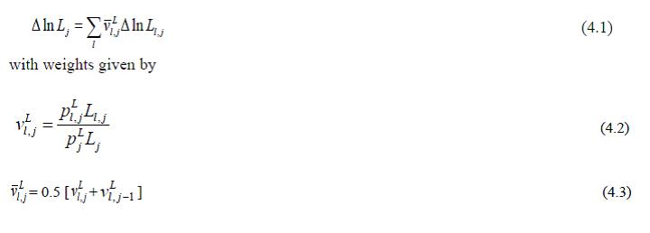 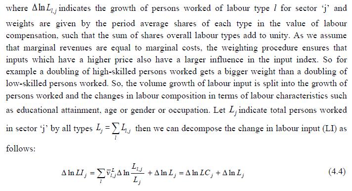 The first term on the right-hand side Δln LCj indicates the change in labour composition and the second term indicates the change in total persons worked in sector ‘j’. It can easily be seen that if proportions of each labour type in the labour force change, this will have an impact on the growth of labour input beyond any change in total persons worked. The index of aggregate labour composition measures the changes in the sex-age-education-occupation composition of the economy. It is the partial index corresponding to all characteristics. The use of this method is, however, data intensive. There is a second approach to the measurement of skill levels. The procedure is to use a simple index of educational attainment to adjust for skill differences. So improvement in educational attainment is adjusted by incorporating average years of schooling as the proxy for skill levels. For example, an index of the form: L* = eas L assumes that each year of schoolings, raises the average worker’s productivity by a constant percentage, ‘a’. Such studies have been carried out for different time periods and for a large number of countries around the world, typically finding a return to each additional year of education in the range of 7 to 12 percent (BCV, 2007). Most of the recent indices of composition of labour input are based on the methodology of Jorgenson, Gollop & Fraumeni (JGF, 1987) and uses the Törnqvist translog index. However, this methodology requires large volume of data. Using this methodology Aggarwal (2004) estimated labour composition for the Indian manufacturing labour force. There are however, lot of disagreements on the use of this methodology in the Indian context, as it assumes the existence of perfectly competitive labour markets where wage rate is the indicator of a person’s marginal productivity. The analysts argue that the observed wage differences may reflect factors other than productivity differences, such as age or gender. Its use is also questioned because data for large segment of Indian labour force- the self -employed is not available. Since the Indian labour market is still not very competitive and there are data weaknesses, therefore the researchers in India have generally avoided applying the JGF methodology. For this reason, most Indian researchers have avoided to account for the differences in age and gender characteristics. However, to account for educational differences they have preferred to exercise either of the two choices- one to use Barrow & Lee (1993) methodology and presume a constant rate of return for education (BCV, 2007) or second is to use the limited information available on wages for few rounds and only for casual and regular employees (Sivasubramonian, 2004) to determine the weights of different types of persons. Bosworth & Collins (2008) assumed a constant annual return of 7 per cent for each additional year of education irrespective of the level of education. The problem with the assumption of uniform returns for each year is that it ignores all variations- across levels of education, over gender, over age groups, over industries, etc. and only includes education. It is thus not able to capture the impact of change in gender composition, age composition (a proxy for experience) and industry composition. The present version of the manual and report now has included some of these characteristics. So a grand labour composition index, an education, an age and a gender labour composition index have been estimated based on JGF methodology using suitable data. The data on employment is essentially derived from the unit level record data of National Sample Survey (NSS) which is made available by NSSO in the form of CD-ROMS for the five quinquennial rounds beginning from 38th. We estimated the number of employed persons according to UPSS as follows:
For extrapolation backward to 1980-81 to 1982-83, the interpolation of the broad industrial classification of 32nd round and 38th round is used. So the estimates from 32nd round are mainly used as control numbers. For the construction of the four labour composition indices we require data on employment and earnings by education, age and gender for the broad sectors and for each of the 27 industries. We distinguish five types of educational categories for broad sectors and three types of educational categories for each of 27 industries because of large data requirement at disaggregate level. While the five education categories used are ‘below primary’, ‘primary’, ‘middle’, ‘secondary & higher secondary’, and ‘above higher secondary’, the three are ‘up to primary’, ‘above primary to higher secondary’, and ‘above higher secondary’. The three age groups used are 14-30, 30-49, above 49 years, and the two gender used are males and females. Table 4.1 below summarizes all this. Therefore the following additional steps have also been performed:
Once the above steps are taken to find out educational distribution of all employed persons in all the six rounds and their corresponding wages, the computation of the labour education index is carried based on the JGF (1987) methodology with 1980-81 equal to 100. The education index is estimated for total persons working in 27 different industries in India for the 38th, 43rd, 50th, 55th, 61st 66th, and 68throunds of NSSO with 1983 (38th round) equal to 100 so as to assess the temporal changes in labour skill. Since the series required is from 1980-81, we have extrapolated it backwards from 1983. The third phase of this project aims to perform some robustness checks and bring out policy implications from the employment trends. Appendix C: Definitions of Employment in NSSO employment & unemployment surveys The surveys of NSSO on employment and unemployment (EUS) aim to measure the extent of ‘employment’ and ‘unemployment’ in quantitative terms disaggregated by various household and population characteristics following the three reference periods of (i) one year, (ii) one week, and (iii) each day of the week. Based on these three reference periods three different measures, termed as usual status, current weekly status, and the current daily status, are arrived at. While all these three approaches are used for collection of data on employment and unemployment in the quinquennial surveys, the first two approaches only are used for the purpose in the annual surveys. Usual principal status: In NSS 27th round, the usual principal activity category of the persons was determined by considering the normal working pattern, i.e., the activity pursued by them over a long period in the past and which was likely to continue in the future. For the identification of the usual principal status of an individual based on the major time criterion, in NSS 27th, 32nd, 38th, 43rd rounds, a trichotomous classification of the population was followed, that is, a person was classified into one of the three broad groups ‘employed’, ‘unemployed’ and ‘out of labour force’ based on the major time criterion. From NSS 50th round onwards, the procedure was changed and the prescribed procedure was a two-stage dichotomous one which involved a classification into ‘labour force’ and ‘out labour force’ in the first stage, and thereafter, the labour force into ‘employed’ and ‘unemployed’ in the second stage. Usual subsidiary status: In the usual status approach, besides principal status, information in respect of subsidiary economic status of an individual was collected in all employment and unemployment surveys. For deciding the subsidiary economic status of an individual, no minimum number of days of work during the last 365 days was mentioned prior to NSS 61st round. In NSS 61st round, a minimum of 30 days of work, among other things, during the last 365 days, was considered necessary for classification as usual subsidiary economic activity of an individual. Current weekly status: It is important to note at the beginning that in the EUS of NSSO, a person is considered as worker if he/she has performed any economic activity at least for one hour on any day of the reference week and uses the priority criteria in assigning work activity status. This definition is consistent with the ILO convention and used by most of the countries in the world for their labour force surveys. In NSSO, prior to NSS 50th round and in all the annual surveys till NSS 59th round, data on employment and unemployment in the CWS approach was collected by putting a single-shot question ‘whether worked for at least one hour on any day during the last 7 days preceding the date of survey’. The information so collected was used to determine the CWS of the individuals. This procedure was criticized for being not able to identify the entire workforce, particularly among the women. It was then decided to derive the CWS of a person from the time disposition of the household members for the 7 days preceding the date of survey. The procedure was used for the first time in NSS 50th round. It is seen that the change in the method of determining the current weekly activity had resulted in increasing the WPR in current weekly status approach - more so for the females in both rural and urban areas than for males. The trend observed in NSS 50th round in respect of the WPR according to CWS suggested continuing with the procedure for data collection in CWS in NSS 55th and NSS 61st rounds. Current Daily Status Current Daily Status (CDS) rates are used for studying intensity of work. These are computed on the basis of the information on employment and unemployment recorded for the 14 half days of the reference week. The employment statuses during the seven days are recorded in terms of half or full intensities. An hour or more but less than four hours is taken as half intensity and four hours or more is taken as full intensity. An advantage of this approach was that it was based on more complete information; it embodied the time utilisation, and did not accord priority to labour force over outside the labour force or work over unemployment, except in marginal cases. A disadvantage was that it related to person-days, not persons. Hence it had to be used with some caution.
Chapter 5: Capital Input Series at the Industry Level This chapter outlines the methodology employed to estimate capital services for the 27 industries in the India KLEMS database version 2015. Following an overview of the theoretical method developed by Jorgenson and Griliches (1967), and outlined in Jorgenson, Gollop and Fraumeni, (JGF, 1987), the Chapter discusses the specific empirical approaches we follow to implement these methods within the constraints of data availability for Indian industries. For the measurement of capital services we need capital stock estimates for detailed asset types and the shares of each of these assets in total capital remuneration. Using the Törnqvist approximation to the continuous Divisia index under the assumption of instantaneous adjustability of capital, aggregate capital services growth rate is derived as a weighted growth rate of individual capital assets, the weights being the compensation shares of each asset, i.e. 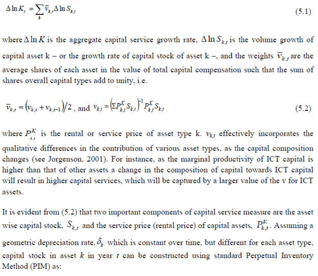  Since our measure of capital input takes account of asset heterogeneity, it was essential to obtain investment data by asset type. We distinguish between 3 different asset types – construction, transport equipment, machinery (includes ICT and non-ICT machinery).22 We exploit multiple sources of information for the construction of our database on capital services. This includes the National Accounts Statistics (NAS) that provide information on broad sectors of the economy, the Annual Survey of Industries (ASI) covering the organized manufacturing sector, the National Sample Survey Organizations (NSSO) rounds for unorganized manufacturing and input-output tables. Even though we use multiple sources of data, our final estimates are fully consistent with the aggregate data obtained from the NAS. In addition, our approach to capital measurement is consistent with international practices such as the EU KLEMS23, which ensures the possibility of international comparisons. In what follows we discuss the various sources of data for asset wise investment and the construction of the relevant variables, in detail. (a) Asset-wise investment for broad sectors of the economy Industry-level estimates of capital input require detailed asset-by-industry investment matrices. NAS provides information on aggregate capital formation by industry of use for 9 broad sectors, which, nevertheless, was not sufficient for our purpose. Therefore, we have collected more detailed data on assets and industries from the CSO.24 This is the data underlying the published aggregate gross fixed capital formation by the broad industry groups, separately for public and private sectors. For those sectors for which the investment matrices were not available from CSO, we gather information from other sources (e.g. ASI for organized manufacturing and NSSO surveys for unorganized manufacturing) and benchmark it to the aggregate investment series from the National Accounts. Table 5.1 provides an overview of asset types available in NAS and their corresponding asset types used in our study.
Total investment in each asset category is calculated as the sum of private and public sector investment in each asset. Investment in transport equipment is not available separately for private sector. We tried several approaches to impute the private sector transport equipment data. The first was to use the share of transport equipment in non-departmental enterprises. More specifically, we apply the non-departmental enterprise transport equipment to machinery & equipment (including transport equipment) ratio to machinery & equipment in private sector for each industry to obtain industry wise transport equipment for private sector. We take non-departmental enterprise only, rather than the entire public sector, as it may be more realistic as it consists of public sector companies and statutory corporations, excluding administrative sector. However, the sum of industry estimates generated by this approach was not consistent with the reported aggregate private sector transport equipment. Therefore, we take a second step here, which is to use the industry distribution from this series and apply it to the published total private sector transport equipment data. The estimated transport equipment is then subtracted from each industry’s total machinery & transport equipment data, to obtain machinery in private sector as a residual. However, this approach generates many negative numbers in transport equipment in private sector, particularly in transport services. Therefore, we follow a third approach, which is what we finally use in the database. We first distribute the NAS total machinery in the private sector using the industry distribution of machinery and transport equipment. These estimates are then subtracted from each industry’s total machinery & transport equipment data to obtain the transport equipment investment in the private sector industries. (b) Asset-wise investment for non-NAS sectors NAS provides data only for 9 broad sectors, while we have 27 industries, which necessitated further splitting of some of the NAS sectors. This includes aggregate manufacturing (registered and unregistered separately) with 13 sub-sectors; other services into 4 sub-sectors; and real estate activities and business services into 2 sub-sectors. The manufacturing sector investment data was disaggregated into 13 subsectors at the 2 digit level of NIC 1998 using ASI and NSSO data, which will be discussed in detail subsequently. Investment series in service sector has been split into sub-sectors using two alternative approaches–value added shares, and capital/labour ratio in the higher aggregate industry. However, the final data used are based on value-added shares, as a sensitivity analysis did not show a significant difference between the two. In order to split the aggregate capital formation in organized manufacturing sector into 13 study sectors, we use the Annual Survey of Industries. However, the published data does not provide any asset wise investment information; it consists of only the aggregate capital formation or the book value of fixed capital. Most studies in the past have measured gross investment as the difference between book value of asset in period t and in period t-1 and add depreciation in period t to that. This approach has the deficiency of comparing two different samples reported in two different years, where the number of firms/factories might be different. In particular, while using this approach at industry level, for detailed asset categories, it might generate massive negative investment. We follow an alternative approach, following ASI’s definition of gross fixed capital formation (GFCF). ASI defines GFCF as actual additions (newly purchased, second hand and own construction) minus deductions plus depreciation adjustment for discarded assets during the year. This approach is based on a single year’s sample and helps to avoid potentially huge negative investment series, and is also consistent with published ASI GFCF series. The yearly detailed volumes beginning 1964-65 were used to derive the gross fixed capital formation by asset type directly. For the years 1964-1978, the relevant data are obtained from published detailed volumes. For the period, 1983-84 to 2004-05 ASI has generated detailed tables from Block C of ASI schedule that contain data on fixed assets. Data for missing years are interpolated using the changes in investment using book value method. Table 5.2 provides an overview of the asset categories available in ASI, and the relevant asset categories in our study to which they are attributed. Though ASI provides investment in land, for reasons of NAS consistency we exclude it from our database. Once investment in each of these assets and industries are generated using ASI data, we apply this industry-asset distribution to the published aggregate NAS GFCF series for organized manufacturing sector. It may also be noted that from 1960-61 to 1971-72, ASI data are for the census sector and from 1973-74 onwards they are for the factory sector. In order to make these two series comparable over years, we convert the data prior to 1972 to factory sector using the factory/census ratio in 1973. Thus, after these adjustments, we obtain investment data for 13 manufacturing sectors, by asset types, consistent with the NAS aggregate. The data required for creating the gross investment series for the 13 sectors of the unorganized manufacturing sector are obtained from various rounds of NSSO surveys on unorganized manufacturing. We use 4 rounds of NSSO surveys that cover the period 1989-2006. These are 45th round (1989-90), 51st round (1994-94), 56th round (2000-01) and 62nd round (2005-06). Unit level data has been aggregated to 13 industries using the appropriate concordance tables. NSSO provides net addition to owned assets during the reference year within the block of fixed assets, and we use this as a measure of our investment. Asset classification in NSSO has changed over various rounds, and therefore, we have tried to match these with our classification as shown in Table 5.3. The investment series arrived at for four rounds were interpolated to obtain the annual time series of unorganized gross fixed capital formation by asset type. As in the case of registered sector, once the investment by asset types across industries are constructed, the asset-industry distribution is applied to the published NAS aggregate GFCF in unregistered manufacturing to obtain NAS consistent GFCF by asset type and industries. (c) Investment Prices by Asset Types In order to compute asset wise capital stock using PIM (equation 5.3) and rental price (equation 5.4), we require asset wise investment price deflators. Since CSO has provided us with investment data by industries and assets both in current and constant prices, we could derive the price deflators with base 2004-2005. These deflators are directly used for all the three asset categories we have. (d) Initial Stock, Depreciation Rates and Rate of Return As is evident from equations 5.1 to 5.4, our estimates of capital input require time-series data on asset wise capital stock. Capital stock has been constructed using perpetual inventory method (PIM), where the capital stock (S) is defined as a weighted sum of past investments with weights given by the relative efficiencies of capital goods at different ages, which requires data on current investment by asset types, investment prices by asset types and depreciation rate. Also, for the practical implementation of PIM to estimate asset wise capital stock, we require an estimate of initial benchmark stock (see Erumban, 2008b for an in-depth discussion on this issue). NAS provides estimates of net capital stock since 1950 for all the broad sectors in its Statement 17: Net Fixed Capital Stock by industry of use. We take the NAS estimate of real net capital stock in 1950 (in 1999-2000 prices) as our benchmark stock for all non-manufacturing sectors, and for manufacturing sectors the same is taken for the year 1964.26 However, since the NAS estimate is available only for broad sectors and for aggregate capital, we use our industry-asset distribution of GFCF in order to create net fixed capital stock estimates by asset type for all the 27 sectors. NAS also provides detailed tables on assumed life of assets used for computing capital stock, for private units, administrative units as well as departmental and non-departmental units by asset types.27 We use these estimates of lifetime to derive appropriate depreciation rates for non-ICT assets, using a double declining balance rate. We assume 80 years of lifetime for buildings, 20 years for transport equipment, and 25 years for machinery and equipment. The final depreciation rates used in the study are given in Table 5.4 by asset type. Subsequently, we build our capital stock series by asset types for all the 27 industries using our GFCF series from 1950 (1964) onwards for the non-manufacturing (manufacturing) sectors. Our measure of capital input is arrived using equation (5.1), for which we also require estimates of rental prices (see equation 5.4). Assuming that the flow of capital services is proportional to the capital stock at individual asset level, aggregate capital flows can be obtained using a translog quantity index by weighting growth in the stock of each asset by the average shares of each asset in the value of capital compensation, as in (5.1). The rate of return (i) in equation (5.4) represents the opportunity cost of capital, and can be measured either as internal (or ex-post) rate of return, or as an external (ex-ante) rate of return.28 This issue will be addressed in the further revisions of the data. The present version of the database uses an external rate of return, proxied by average of return on government securities and prime lending rate obtained from the Reserve Bank of India29. Therefore, we use a real rate, which is net of capital gain. Hence, the capital gain component in equation (5.4) is excluded while estimating rental price using external rate of return, obtaining  Where i* is the real rate of return, nominal interest rate adjusted for CPI inflation rate. (e) Investment by assets and industries for years after 2013 CSO does not have data on investment by assets and industries that corresponds to the India KLEMS classifications, for years after 2012-2013. Therefore, we had to do some imputations to extend the capital stock and capital service estimates for 2013-2014 and 2014-2015. National accounts provides data on total gross fixed capital formation (GFCF) in two asset types, construction and total equipment (i.e. sum of transport equipment and machinery) for the aggregate economy. We use this data as the benchmark to impute sectoral investment by asset type as follows. First we split the total equipment investment into machinery and transport equipment as: Ii,t = Si,2012 • IEQ,t where Ii,t is the total economy investment in asset i (for i = 1,…,2, i.e. transport equipment and machinery) in year t (for t > 2012-2013) and Si,2013 is the share of asset i in total machinery and equipment investment in 2012-2013. This helps us obtain total economy investment in three asset types, machinery, transport equipment and construction separately. Subsequently these three asset types are distributed across industries as: Ii,j,t = Vi,j,t • Ii,t where Ii,j,t is the investment in asset i (i=1,…,3; construction, machinery and transport equipment), Vi,j,t is the share of industry j in total investment in asset i in year t. This is obtained as 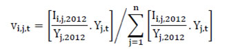 Where Ii,j,2012 is the investment in asset i in industry j in 2012-2013, Yj,2012 is the gross value added in industry j in 2012-2013 and Yj,t is the gross value added in industry j in year t (for t > 2012-2013). Chapter 6: Intermediate Input Series at the Industry Level In this section we describe the basic approach we have used to derive the volume series of intermediate inputs namely – energy input (E), material input (M) and services input (S). This breakdown of intermediate inputs can be used for extending the growth accounting exercises, but also convey interesting information about changing pattern in intermediate consumption ( see e.g. JHS 2005, chapter 4) The methodology for measuring industry output, intermediate inputs and value added was developed by Jorgenson, Gallop & Fraumeni (1987) and extended by Jorgenson (1990 a). The cornerstone of this approach is a time series of input-output (IO) tables which gives the flows of all commodities in the economy, as well as payments to primary factors. Every commodity is accounted for, whether produced by a domestic source or imported, and every use is noted, whether purchased by an industry or by a final demand element. All payments to factors of production i.e. labour and capital is accounted for so that all income elements of GDP are included. The methodology of constructing time series on energy, material and services inputs for the European economy has been elucidated in Timmer et al. (2010, Chapter 3). Following a similar approach as explained in Jorgenson et al. (2005, Chapter 4) and Timmer et al. (2010, Chapter 3), the time series on intermediate inputs for the India KLEMS project have been constructed. Definition of EMS: As in EU KLEMS, this study identifies three main categories of Intermediate inputs. They are classified as follows:
Intermediate Inputs are broken down into energy, material and services, based on input-output transaction tables using a standard NIC product classification. The following five energy types (and products) have been classified as the Energy input.
The following fourteen input items have been classified as the Service input
All other intermediate inputs barring the above mentioned nineteen inputs are classified as material input. The key building block for constructing time series on intermediate inputs at current prices, as explained in Jorgenson et al. (2005, Chapter 4), is the input-output transaction tables, that is, the inter-industry transaction tables that provide a description of which industries produce each product and which industries use them. The input-output table gives the inter-industry transactions in value terms at factor cost presented in the form of commodity x industry matrix where the columns represent the industries and the rows as group of commodities, which are the principal products of the corresponding industries. Each row of the matrix shows in the relevant columns, the deliveries of the total output of the commodities to the different industries for intermediate consumption and final use. The entries read down industry columns give the commodity inputs of raw materials and services, which are used to produce outputs of particular industries. The column entries at the bottom of the table give net indirect taxes (NIT) (indirect taxes – subsidies) on the inputs and the primary inputs (income from use of labour and capital), i.e., Gross Value Added (GVA). As the IOTT is in the form of commodity x industry matrix, the row totals do not tally with the column totals. The difference between each column and the corresponding row totals is due to the inclusion of the secondary products, which appear particularly in the case of manufacturing industries. This is so because by-products are also manufactured by industries in addition to their main products. Thus, while determining the entries in the rows, a by-product of an industry is transferred to the sector (commodity row), whose principal product is the same as the by-product under reference. The columns, however, show the total of principal products and by-products of each industry. All the entries in the IOTT are at factor cost, i.e. excluding trade and transport charges and NIT. The Input Flow Matrix at factor cost, published by CSO, for 1978 is a 60 x 60 matrix. The absorption matrices for 1983, 1989, 1993 and 1998 have 115 sectors. However a detailed 130 sector absorption (commodity x industry) matrix for the Indian economy has been published from 2003-04 onwards. The scheme of sector classification adopted in IOTT 2013-14, IOTT 2007-08 and IOTT 2003-04 vis-à-vis, IOTT 1983-84, IOTT 1989-90, IOTT 1993-94 and 1998-99 has undergone significant change with the disaggregation of some of the sectors, which have become significant in early 2000s.
The methodology for computation of intermediate input series for 27 Industries from 1980-2014 at current and constant prices is explained in steps. Step 1: Concordance is done between IOTT and study industries
Step 2: Obtaining estimates for Material, Energy and Service Inputs for 27 Industries, in benchmark years
Thus, for each of the benchmark year, estimates are obtained for material, energy and service inputs that has been used to produce gross output in the 27 different India KLEMS Industries. Step 3: Projecting a time series (1980 to 2014) of proportions of Material, Energy and Service Inputs in Total Intermediate Inputs for each of the 27 industries
Step 4: Consistency with NAS The projection of intermediate input vector, using IOTT in Step 3 needs to be consistent with the estimated output from NAS.
1. For Benchmark years: Ratio of Total Intermediate inputs from NAS to that from IOTT is adjusted proportionately to the absolute value of Energy Inputs/Material Inputs/Service Inputs obtained from IOTT. 2. For Intervening Years: The interpolated proportions of energy inputs, material inputs and services inputs obtained from IOTT, is applied directly to the total intermediate inputs from NAS to get each inputs share. Two examples have been given below for the construction sector: In the examples above, we can see that the total value of intermediate input exactly matches the gap between Gross output and Value added. Similar adjustments have been made to construct the input series for all the other 27 study industries from 1980-2014. For every benchmark year where IOTT is available adjustment ‘A’ has been done. For every non-benchmark year, where IOTT is not available and an intermediate input vector has been projected, adjustment ‘B’ has been done to generate the comprehensive time series of Intermediate inputs consistent with the official National Accounts. Steps 1-4: This gives a time series of Material, Energy, and Service Inputs for 27 study Industries from 1980 to 2014 at current prices. Steps 5 and 6 below, explain the methodology for computation of Intermediate Input Series for 27 study Industries from 1980-2014 at constant price. The approach followed here is to first form the aggregates of materials, energy and services at current price for each study industry from the benchmark Input-Output tables and then develop deflators of Materials, Energy and Service Inputs for each of the 27 study Industries separately. Step 5: Constructing Deflators of Materials, Energy and Service Inputs for 27 study Industries separately
Step 6: Computing Time Series on Intermediate Input for 27 study Industries from 1980-2014, Constant prices
Thus we have a time series of material, energy and service inputs for 27 study industries at constant prices. Firstly, Input-Output transaction tables are generally available on a five year interval period and this necessitates interpolation and assumption of constant shares in some cases to construct the entire time series of EMS from 1980 to 2014. Secondly, unlike studies using detailed survey data, we have to assume that all buyers pay the same price for each commodity because there is no information about price divergences. Thirdly, The estimated time series of Intermediate Inputs at constant price will not be consistent with the intermediate input of NAS at constant price i.e. the deflated value of intermediate input cannot match the gap between value added and gross output at constant price from NAS. This is because NAS uses a single deflation method to estimate Gross Value Added and Gross Output at constant price. ‘However, only for one sector – agriculture, the gross output and gross value added, estimated by NAS is double deflated. Therefore only for the agriculture sector the deflated value of intermediate input will exactly match the gap between value added and gross output at constant price. Fourthly, there has been some confusion in the literature on the price concept to be used for intermediate inputs. It is generally acknowledged that the intermediate input weights should be measured from the user’s point of view, i.e. reflect the marginal cost paid by the user. Most studies maintain that purchaser’s price should be used. These prices include net taxes on commodities paid by the user and include margins on trade and transportation (see, for example OECD 2001). However, when trade and transportation services are included as separate intermediate inputs, margins paid on other products should also be allocated to these services. Ideally a distinction should be made between the intermediate product valued at purchaser’s price minus margins and the trade and transportation services valued at margins. This is the approach taken in Jorgenson, Gollop & Fraumeni (1987) and in Jorgenson et al. (2005). However, Timmer et al. (2010, Chapter 3) explains that for the EU KLEMS database, intermediate inputs have been valued at purchaser’s price owing to unavailability of necessary data. Because of the use of purchaser’s price concept the shares of services in intermediate inputs do not include trade and transportation margins. Similarly in practice for the database, the time series of Intermediate Input constructed is at purchaser’s price i.e. it implicitly takes into account the net indirect taxes. The distribution of this net indirect tax between material, energy and services has not been possible because of unavailability of a time series of tax matrix from 1980 to 2014. Chapter 7: Factor Income Share Series at the Industry Level The distribution of income between capital, labour and intermediate inputs, is an important element in growth accounting because income shares under conditions of competitive markets can be used to measure the contributions each factor makes towards output growth. 7.1 Methodology for Measuring Labour Income Share Series Under the assumption of constant returns to scale with two factors of production i.e., labour and capital, the sum of the labour income share and capital income share is 1. The labour income share is defined as the ratio of labour income to GVA. Capital income share is accordingly obtained as one minus labour income share. There are no published data on factor income shares in Indian economy at a detailed disaggregate level. National Accounts Statistics (NAS) of the CSO publishes the NDP series comprising of compensation of employees (CE), operating surplus (OS) and mixed income (MI) for the NAS industries. The income of the self-employed persons, i.e. mixed income (MI) is not separated into the labour component and capital component of the income. Therefore, to compute the labour income share out of value-added, one has to take the sum of the compensation of employees and that part of the mixed-income which are wages for labour. The computation of labour income share for the 27 study industries involves two steps. First, estimates of CE, OS and MI have to be obtained for each of the 27 study industries from the NAS data which are available only for the NAS sectors (see Table 7.1). Second, the estimate of mixed-income has to be split into labour income and capital income for each industry for each year (except for those industries for which the reported mixed income is zero, for instance, public administration). Basis data sources used for the computation of labour income share are NAS, ASI and unit level data of survey of unorganized manufacturing enterprises. These data sources are used to obtain estimates of CE, OS and MI for each of the 27 study industries. For splitting the labour and non-labour components out of the mixed-income of self-employed, the unit level data of NSS employment-unemployment survey are used along with the estimates of CE, OS and MI basically obtained from the NAS. a) Construction of Labour Income Share Series in Gross Value Added The estimation of labour income share for the 27 study industries has been done in two steps, as discussed below. Step 1: Estimation of CE, OS and MI for the 27 study Industries For some industries under study, for instance (i) Agriculture, forestry & logging and fishing, (ii) Mining & Quarrying, (iii) Electricity, gas and water supply and (iv) Construction, the required data are readily available from NAS. For others, the estimates available in NAS have to be distributed across the study industries. In certain cases, the estimates of CE, OS and MI for a particular NAS sector have been distributed across constituent study industries proportionately in accordance with the gross value added in those industries. Estimate of factor incomes for ‘other services’ in NAS, for instance, has been split into estimates for (i) Education, (ii) Health and Social Work, and (iii) Other Community, Social and Personal Services including Renting of machinery and business services, and Private Household with Employed Persons. NAS provides estimates of factor incomes for registered manufacturing and unregistered manufacturing, but not for individual manufacturing industries. The NAS estimates of factor incomes for registered manufacturing have to be split into various manufacturing industries considered in the study (13 in number) using ASI data. The reported CE in NAS for registered manufacturing has been distributed into those 13 industries in proportion to the reported ASI data on emoluments for various industries. In a similar way, using ASI data, the estimate of OS for registered manufacturing has been distributed. Emoluments are subtracted from gross value added for various industries yielding capital income. The share of different industries in aggregate capital income of organized manufacturing indicated by the ASI data is used to split the estimate of OS for registered manufacturing reported in the NAS. The methodology applied for unregistered manufacturing is similar. The published results and unit level data of survey of unorganized manufacturing industries have been used for this purpose. The estimates of wage payments (to hired workers) in different industries have been used to split (proportionately) the estimate of CE in the NAS for aggregate unregistered manufacturing. The estimated wage payment is subtracted from the estimated value added to obtain an estimate of capital income and mixed income of the self-employed in various unorganized manufacturing industries. The estimate of MI provided in NAS for unregistered manufacturing has then been proportionately distributed across industries using the estimate of capital income and mixed income of the self-employed in various industries that could be formed on the basis of published results and unit level data of survey of unorganized manufacturing industries. Unlike the ASI data for organized manufacturing, the data for unorganized manufacturing enterprises are available for only select years. The proportions mentioned above could therefore be computed only for those select years (data for five rounds have been used; these are for 45th round (1989-90), 51st round (1994-95), 56th round (2000-01), 62nd round (2005-06) and 67th round (2010-11)). It has accordingly been necessary to resort to interpolation/ extrapolation to obtain the relevant proportions for other years. Step 2: Splitting of MI into Labour Income and Capital Income As explained above, the income share of labour is computed as: 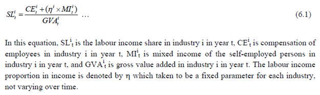 The derivation of the GVA series for different industries has been briefly explained in Chapter 2. The derivation of CE and MI series has been explained in step I above. Therefore, only the estimation method of ƞ needs to be described. The estimation of ƞ has been done with the help of NSS survey-based estimates of employment of different categories of workers (number of persons and days of work) and wage rates (which has been described briefly in chapter 4) coupled with estimates of MI, basically obtained from the NAS. Two approaches have been taken to get an estimate of ƞ, and the labour income share series for different industries finally adopted in the study makes use of an average of the estimates of ƞ obtained by the two approaches. In the first approach, an estimate of labour income of self-employed workers has been made for each study industry for five years, 1983-84, 1987-88, 1993-94, 1999-00, 2004-05, 2009-10 and 2011-12 on the basis of the estimated number of self-employed, wage rate of self-employed and the number of days of work per week. The industry-wise estimates of number of self-employed, wage rate of self-employed and the number of days of work per week have been made from unit records of NSS employment-unemployment survey (major rounds), as explained in chapter 4 above. The estimates of the number of self-employed, wage rate of self-employed and the number of days of work per week provide an estimate of the annual labour income of self-employed workers which is divided by the mixed-income of self-employed (derived from NAS) to get an estimate of ƞ. For five industries, the ratio in question has been computed and applied. For the other 22 industries, the ratio in question has been computed after clubbing the industries into 11 industry groups.30 In the latter case, a common ratio computed for group of industries has then been applied to constituent industries. The list of industries or industry groups for which ƞ has been estimated is given in table 7.2. In the second approach, the NSS data are used to compute the following ratio: the ratio of labour income of self-employed workers to the labour income of regular and casual workers. Let this be denoted by θ. Then, the estimate of CE provided in the NAS is multiplied by θ to obtain an estimate of the labour income component out of the MI reported in the NAS. The labour component of MI divided by total MI gives an estimate of ƞ. In case the estimated labour component of MI exceeds the estimate of MI, the estimate of ƞ has been taken as unity. Examining the estimates obtained by the first approach, it was found that the estimated labour income share out of mixed-income varied significantly among the estimates for the seven years for which the ratio in question has been estimated. The estimates of ƞ obtained by the second approach has the problem that in a number of cases, the estimated labour component of MI exceeds the estimate of MI given in the NAS, and therefore ƞ is taken as one. The method finally adopted is as follows: (a) The average value of ƞ has been computed for each industry or industry group by taking the estimates for the years 1983-84, 1987-88, 1993-94, 1999-00, 2004-05, 2009-10 and 2011-12. This has been done separately for the estimates based on approach-1 and those based on approach-2. (b) The estimates of ƞ obtained for each industry or industry group by the two approaches have then been averaged. (c) Having obtained an estimate of ƞ, equation 6.1 given above has been applied to compute the labour income share. b) Construction of Factor Income Share Series in Gross output The income share of labour, capital and intermediate inputs in Gross output has been computed using the following steps:
The splitting of unorganized sector factor incomes into individual industries has been done using unorganized survey results. The proportions computed for 1983-84 has been applied for the period 1980-81 to 1983-84. While there were surveys of unorganized manufacturing enterprises in 1978-79 and 1984-85, the survey results have not been used for estimation of factor incomes in different industries of the unorganized manufacturing sector. An attempt will be made to use survey data for the years 1978-79 and 1984-85 rather than applying the proportions computed for 1989-90 to factor income data for earlier years. In case of KLEMS data series, we have used CE, OS and MI data from NAS. As NAS provides information on CE and OS for aggregate registered manufacturing. So we distribute it among 13 registered manufacturing industries using ASI information. Similarly for unorganized manufacturing we have information on CE and MI. so we distribute it using NSSO information. And then add up the registered and unregistered portion to get overall manufacturing CE, OS and MI. In case of organized and unorganized manufacturing data set, we use Emoluments/GVA from ASI as labour income share for organized manufacturing industries. And Emoluments/GVA for NDME+DME as labour income share for unorganized manufacturing. Chapter 8: Growth Accounting Methodology This chapter deals with the methodology of measurement of total factor productivity (TFP) growth for individual industries in the KLEMS framework and the aggregation from industry-level productivity measures to measures for broad sectors and the economy as a whole. The methodology of analysis of sources of gross output growth at the individual industry level and sources of GVA (Gross Value Added) or GDP growth at the broad sector level and economy level will also be presented in this chapter 8.1 Methodology for Measuring Productivity Growth at the Industry level The production function Our measurement of TFP growth for different industries of the Indian economy is based on a gross output production function for each industry j: Y = f(L(L1,…Ln), K(K1…Km), E(E1….Es), M(M1 …Mu), S(S1 … Sv), T) (8.1) Y is industry gross output, L is labour input, K is capital input and E, M and S are intermediate inputs-namely energy, material and services and T is an indicator of technology for industry j. All variables are indexed by time (t subscript is suppressed). There are several things to note about the production function- (1) all variables are aggregates of many components that have been discussed in the earlier report/chapters; (2) we assume that the industry production function is separable in these aggregates; (3) time (indicator of technology) enters the production function symmetrically and directly with inputs. An important feature of the gross output approach is the explicit role of intermediate inputs. In our study, we have considered three intermediate inputs - energy, material and services and this is important as we may find that intermediate inputs are the primary component of some industries outputs.31 Failure to quantify intermediate inputs leads us to miss both the role of key industries that produce intermediate inputs and the importance of intermediate inputs for the industries that use them. In order to estimate the production function at constant prices, the industry level price data is used for output, capital, labour and intermediate inputs, e.g., PYj; PLj, PKj; PEj. PMj, PSj. We assume that all industries face the same input price. The industry price of an input varies across industries due to compositional effects as industries expend different shares of their investment on each type of asset. The same is true for all inputs. 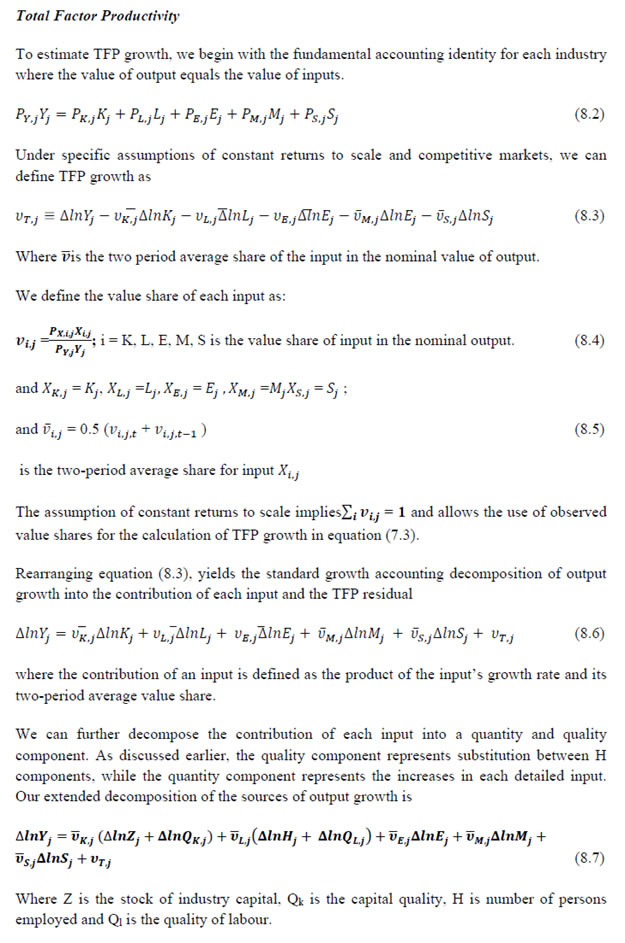 8.2 Methodology for Aggregation across Industries In the analysis presented in the above section, gross value of output (GVO) is taken as the measure of output of an industry and TFP growth was estimated using the gross output function framework in which capital, labour, materials, energy and services are taken as five inputs (in the case of agriculture, land was included among inputs). The Törnqvist index is applied to estimate TFP growth for each year during 1980-81 to 2014-15, which yielded an index of TFP for each industry for that period, permitting estimation of trend growth rate in TFP for the period under study (1980-81 to 2014-15). The method of estimation of TFP growth for individual industries described in section 7.1 cannot be readily applied to a higher level of aggregation. The main problem is that gross value of output cannot be added across industries to generate a measure of output at a higher level of aggregation, say for the economy or of any of the broad sectors. It becomes necessary therefore to consider appropriate methods of aggregation across industries consistent with the gross output function specification of technology at the individual industry level. It is needless to say that one has to use the concept of value added to define an appropriate measure of output at the economy or broad sector level, but even here there are important issues of aggregation, i.e. how value added in different industries should be combined. A very useful discussion of the issues involved is found in Jorgenson et al. (2005). There are three approaches to estimating TFP growth at an aggregate level. This is discussed in detail in Jorgenson et al. (2005). The first approach is called aggregate production function approach. This approach assumes the existence of an aggregate production function (say, at the level of the economy or at the level of manufacturing or services sector). An essential condition is that the production function be separable in primary inputs. Let the production function for a particular industry be defined as: Y =f(X, K, L, T), (8.8) where Y denotes gross output, X intermediate input (in turn a combination of materials, energy and services), K capital input, L labour input and T time (representing technology). Then, the concept of value-added requires the existence of a value-added function which in turn requires that the above production function be separable in K, L and T, i.e. the production function should take the following form: Y =g(X, V(K, L, T)). (8.9) In this equation, V (.) is the value-added function. V denotes value added. Besides the condition of separability of the production function described above, a number of highly restrictive assumptions have to be made for the aggregate production function approach. These include: (a) the value-added function is the same across all industries up to a scalar multiple, (b) the functions that aggregate heterogeneous types of labour and capital must be identical in all industries, and (c) each specific type of capital and labour receives the same price in all industries. With these assumptions made, real value added at the aggregate level becomes a simple addition of real value added in individual industries. In notation,  where Vi is value added in the i'th industry and V is the aggregate value added. Given aggregate value added and somewhat similarly defined aggregate capital and labour input, TFP growth at the aggregate level can be computed. The second approach to aggregation is the aggregate production possibility frontier approach. It also needs the separability condition described in equations 7.8 and 7.9 above, as in the case of the aggregate production function approach. The main difference between the aggregate production function approach and the aggregate production possibility frontier approach is that the latter relaxes the assumption that all industries must face the same value-added function. Thus, the price of value added is no longer assumed to be the same across industries. The implication is that the aggregate value added from the aggregate production possibility frontier is given by the Törnqvist index of the industry value added as:  In this equation, wi is the share of industry i in aggregate value added in nominal terms. Thus, defining PV,i as the price of value added in industry i and Vi as the real value added in industry i, the share in question may be defined as:  and the two-period average is defined as:  Since each industry is subject to a production function separable in capital, labour and technology, as defined in equation7.9, real gross output, real value of intermediate inputs and real value added of industry i in a particular year t should satisfy the following relationship:  In this equation, uV and uX are the shares of value added and intermediate inputs in the gross value of output in nominal terms. Given data on growth in gross output and growth in intermediate input of a particular industry, the above equation yields the growth in real value added of that industry. TFP growth from the aggregate production possibility frontier may be defined as follows:  In this equation K and L are aggregate capital input and labour input respectively, and VK and VL are value shares (or income shares) of capital and labour respectively. If one maintains the assumption that each specific type of capital and labour input has the same price in all industries, then each type of capital (labour) can be summed across industries and then a Törnqvist index can be constructed to yield aggregate capital (labour) input. Alternatively, different types of capital input can be combined using a Törnqvist index into total capital input used in an industry and then industry level growth in capital input can be combined with the help of a Törnqvist index to obtain growth in capital input at the aggregate level. In a similar manner, the growth in aggregate labour input can be computed. The third approach to measuring the TFP index at a higher level of aggregation is to apply direct aggregation to industry level estimates. This maintains the industry level production accounts as the fundamental building block and begins with industry level sources of growth. Of the three approaches described here, this is the least restrictive in terms of the assumptions involved. The following equation expresses the relationship between aggregate value-added growth and the growth in capital and labour inputs and TFP in individual industries:  In this equation, vK is the value share of capital in gross output, VL is the value share of labour in gross output, VV is the share of value added in gross output, and Wi is the share of industry i in aggregate value added in nominal terms. The bars indicate that the average of two periods, t and t-1, are to be taken. The last term in equation 7.16 is:  This is the Domar aggregation of TFP growth rates at individual industry level. Note that it is weighted average of industry level TFP growth rates. But, the weights add up to more than one. The data constructed for gross value added and gross output, labour input, capital inputs, intermediate inputs and factor income shares (Chapters 2, 3,4,5,6 and 7 respectively), are used to estimate TFPG during the period 1980 to 2014. Labour input is measured using total person worked (see, Chapter 4 for the detailed discussion). The series on growth rate in capital services is taken from Chapter 5. 1 Kanhaiya Singh and M. R. Saluja (2016), Input-Output Table for India, 2013-14, Working Paper no WP-111, National Council of Applied Economic Research, New Delhi. 2 Kanhaiya Singh and M. R. Saluja (2016), Input-Output Table for India, 2013-14, Working Paper no WP-111, National Council of Applied Economic Research, New Delhi 3 Timmer, M.P, Mahony, M. and van Ark, B.(2007). The EU KLEMS growth and productivity accounts: an overview. Mimeo University of Groningen & University of Brinmingham, 4 Readers can refer to India KLEMS Data Manual Version 2013 for the data set released by RBI on its website in June 2014. 5 From both aggregated 9 NAS sectors Gross Domestic Product by economic activity statement along with the disaggregated statements of these 9 NAS sectors. 6 It uses NAS Series 2004-05 for more recent years. 7 Kanhaiya Singh and M.R. Saluja (2016), Input-Output Table for India, 2013-14, Working Paper no WP-111, National Council of Applied Economic Research, New Delhi 8 The principal components of Manufacturing n.e.c. are Manufacturing of jewellery and related articles, Manufacture of musical instruments, Manufacture of sports goods, Manufacture of games and toys and other manufacturing. 9 See Himanshu (2011) for a discussion on many issues associated with the NSSO employment surveys. 10 The coverage and the sample size of thin rounds is different from major rounds. 11 Problems in using UPSS are: The UPSS seeks to place as many persons as possible under the category of employed by assigning priority to work; no single long-term activity status for many as they move between statuses over a long period of one year, and Usual status requires a recall over a whole year of what the person did, which is not easy for those who take whatever work opportunities they can find over the year or have prolonged spells out of the labour force. 12 In EU-KLEMS changes in labour composition has been measured by including employment class, gender, age and education (Timmer,op cit; p64) and only 3 categories of education defined as high skilled, medium skilled and low skilled have been taken. This concept of labour composition is refereed as ‘labor quality’ by Jorgenson. It is recognized (Timmer; op cit; p84) that the categorization may lead to biases in the aggregate composition adjustment if employment trends and wage share differ within categories. These education categories generally correspond to- up to Primary education, above Primary to Hr Secondary education and above Hr Sec or College education. Due to data limitations in India we have measured changes in labour composition only by changes in education profile of labour; hence named it labour education index. Therefore it became necessary to have a more detailed classification of education to capture the changes in skill composition of labour in India. For comparison, we estimated the changes in labour composition based on three education categories also and found that for the total economy the annual trend growth in labour education index is 1.16 percent as compared to 1.25 percent based on five education categories. 13 This procedure has been advocated by NSSO itself and has been consistently adopted by almost all researchers. 14 A very lucid description of the same is given by Sivasubramonian (2004). 15 Appendix Table 1 provides the details about the Census Population, WFPR by UPSS, and persons employed in each of the EUS rounds used in the study. 16 Aggregate input is measured as a translog index of its individual components. Then the corresponding index is a Törnqvist volume index (see Jorgenson, Gollop and Fraumeni 1987). For all aggregation of quantities we use the Törnqvist quantity index, which is a discrete time approximation to a Divisia index. This aggregation approach uses annual moving weights based on averages of adjacent points in time. The advantage of the Törnqvist index is that it belongs to the preferred class of superlative indices (Diewert 1976). Moreover, it exactly replicates a translog model which is highly flexible, that is, a model where the aggregate is a linear and quadratic function of the components and time. 17 Although census population is available only decennially, we used the interpolated population figures for the mid-year survey periods [Visaria, (1996) for 1977-78 (Jan) and 1987-88 (Jan); Sundaram, (2007) for 1983 (July), 1993-94 (Jan), 1999-00 (Jan) and 2004-05 (Jan)] and from NSSO (2010) for Jan 2010 and Jan 2012. 18 In EU KLEMS (Timmer, op cit; p 67) it is assumed that the earnings is equal to the earnings of ‘regular' employees. 19 The details of the function can be obtained from the Stata software and from Appendix. 20 Asset prices are used in the aggregation of capital stock. However, it is the price of the capital service that must be used in aggregating capital services (see Jorgenson and Griliches, 1967; Diewert, 1980) as it is the services delivered by capital goods that are used in the production process,. Jorgenson and Griliches (1967) have shown that these two prices are related; the asset prices are the discounted value of all future capital services. They are not proportional though, as there are differences in replacement rates and capital gains among different capital assets. 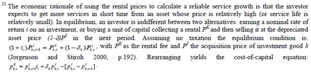 22 This version of the database does not make a distinction between ICT and non-ICT assets, as the industry level data on ICT assets are weak. An attempt to estimate aggregate economy level ICT capital can be found in Erumban and Das (2015). 23 See O’ Mahony and Timmer (2009) for a description of EU KLEMS database 24 This data is not publicly available. However, CSO has been kind to compile this data for the India-KLEMS project. 25 In some years transport equipment was provided as part of the machinery and equipment, categorized as ‘tools, transport equipment and other fixed assets’. In such cases, we use transport/tools, transport and other fixed asset ratio in the nearest year to separate transport equipment. 26 This choice is driven by the fact that the first year of availability of ASI data is 1964-65. 27 National Accounts Statistics-Sources and Methods, Chapter 26, CSO (2007) 28 We do not intend to delve into the controversies over the use of internal vs. external rate of return in the context of productivity measurement. Rather, given that this is the first version of our data, we use the external rate and in a later stage, we will also use internal rates. See Erumban (2008a and b) for a discussion on these issues. 29 Reserve Bank of India, Handbook of Indian Statistics, Annual volumes. 30 The estimation is done at group level rather than individual industries on the consideration that the group level estimates will be more reliable. 31 Consider, the semi conductor (SC) industry, which is a key input to the computer hardware industry. Much of the output is invisible at the aggregate level because semi conductor products are intermediate inputs to other industries rather than deliverables to final demand- consumption and investment goods. Moreover, SC plays a role in the improvements in quality and performance of other products like-computers, communication equipments and scientific instruments. Failure to account for them leads us to miss the role of key industries that produce intermediate inputs and importance of intermediate inputs for the industries that use them. [Jorgenson, Ho and Stiroh (2005), Productivity, volume 3]. |
|||||||||||||||||||||||||||||||
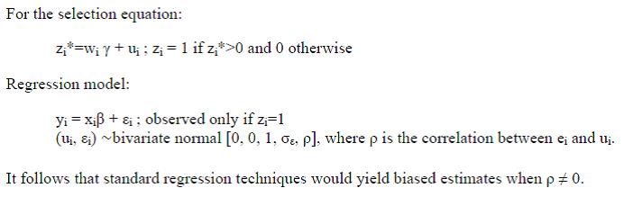
Measuring Productivity at the Industry Level - The India KLEMS Database
|
AUTHORS Deb Kusum Das Abdul Azeez Erumban Suresh Aggarwal Pilu Chandra Das This document describes the procedures, methodologies and approaches used in constructing the India KLEMS database version 2017. This database is part of a research project, supported by the Reserve Bank of India (RBI), to analyze productivity performance in the Indian economy at disaggregate industry level. This work is meant to support empirical research in the area of economic growth. In addition the database is meant to support the conduct of policies aimed at supporting acceleration of productivity growth in the Indian economy, requiring comprehensive measurement tools to monitor and evaluate progress. Finally, the construction of the database would also support the systematic production of reliable statistics on growth and productivity using the methodologies of national accounts and input-output analysis. In its definitive version the India KLEMS research project will include measures of economic growth, employment creation, capital formation and productivity at the industry level from 1980-81 onwards. The input measures will incorporate various categories of capital (K), labour (L), energy (E), materials (M) and services (S) inputs. A major advantage of growth accounts is that it is embedded in a clear analytical framework rooted in production functions and the theory of economic growth. It provides a conceptual framework within which the interaction between variables can be analyzed, which is of fundamental importance for policy evaluation. (Timmer et.al.2007)1. The present document describes the India KLEMS database version 2017. The present version is an extended India KLEMS research project, “Disaggregate Industry Level Productivity Analysis for India- the KLEMS Approach” being undertaken at the Centre for Development Economics, Delhi School of Economics. This one builds on the previous project, which was undertaken at ICRIER, New Delhi2. The Data Manual is intended to guide researchers about the variables (and their construction) used to measure both inputs and total factor productivity (TFP) at the industry level using the dataset. In addition, it is also intended to support national officials statistical agencies in future work on of the productivity database within the agencies. The dataset includes measures of Gross Value Added(GVA), Gross Value of Output (GVO), Labour (L), Capital (K), Energy (E), Material (M), Services (S), Labour Quality (LQ), Labour Productivity (LP) and Total Factor Productivity (TFP) at the industry and economy level from 1980-81 onwards. The database covering the period 1980-81 to 2015-16 has been constructed on the basis of data compiled from CSO, NSSO, ASI, Input-Output tables (I-O tables) and processed according to appropriate procedures. These procedures were developed to ensure harmonization of the basic data, and to generate growth accounts in a consistent and uniform way. Harmonization of the basic data has focused on a number of areas such as industrial classification, aggregation levels. The data base covers 27 industries comprising the entire Indian economy. The industries are shown in Table 1.1 below. The variables in the data set are given in Table 1.2. 1.2 Coverage: Industries and Variables In this section we describe the coverage of the India KLEMS database in terms of industries and variables. In principle, the 36 year period from 1980-81 (1980) to 2015-16 (2015) is covered. At a disaggregated level, database is created for 27 industries. The industrial classification is constructed by building concordance between NIC 2008, NIC 2004, NIC 1998, NIC 1987 and NIC 1970 so as to generate continuous time series from 1980 to 2015. This classification is very close to the International Standard Industrial Classification (ISIC) revision 3. The 27 industries are aggregated to form six broad sectors, namely:
Table 1.1 below provides a listing of the 27 industries, including the higher aggregates. Further the detailed classification and concordance of study industries with NICs is provided in Appendix table A. Table 1.2 provides an overview of all the series included in our database. Measures of capital (K), labour (L), energy (E), material (M) and service (S) inputs as well as gross output (GO), have been constructed using National Accounts Statistics (NAS), Annual Survey of Industries (ASI), NSSO rounds and Input-Output Tables (IO). In building annual time series on gross output, five inputs and factor income shares, various assumptions are made to fill up gaps in industry details and link series over time. As we know that NSSO rounds of unregistered manufacturing, Input Output Transaction Tables, and Employment and Unemployment Surveys by NSSO are available only for certain benchmark years. Thus, the use of information from these data sources necessitates interpolation and assumption of constant shares for building series of output and inputs. The construction of growth accounting series like total factor productivity, labour productivity are based on theoretical models of production and needs additional assumptions that are spelt out in subsequent chapters of the manual. Finally, the Other Series like NDP at factor cost, compensation of employees etc. are additional series which are used in generating the growth accounts and are informative by themselves. Chapter 2: Gross Value Added Series at the Industry Level For an individual firm or industry, productivity measure can be based on a value added concept where value added is considered as an industry’s output and only primary inputs such as labour and capital are considered as industry input. Value added based productivity measures reflect an industry’s capacity to contribute to economy wide income and final demand. In this sense they are valid complements to gross output based measures. This chapter describes the data sources and methodology used to construct the Gross Value Added (GVA) series at current and constant prices for 27 study industries for the period of 1980-81 (1980) to 2015-16 (2015). GVA of a sector is defined as the value of output less the value of its intermediary inputs. This value added created by a sector is shared among the primary factors of production, labour and capital. The National Accounts Statistics (NAS) brought out by the CSO (Central Statistics Office, Government of India) is the basic source of data for the construction of series on gross value added for INDIA KLEMS-industries. NAS provides estimates of GVA (i.e. gross value added) for Indian economy at a disaggregate industry level at both current and constant prices for the period since 1950-51. CSO provide GVA at constant (2011-12) prices onwards 2011-12, and prior to that at constant (2004-05) prices. Up to 2011-12, estimates of GVA at both current and constant (2004-05) prices for all industries are directly obtained from Back Series 2011 and NAS 2014. And onwards 2011-12, estimates of GVA at both current and constant (2011-12) prices for all industries are directly obtained from NAS 2017. GVA series at current and constant (2011-12) prices are extended backwards up to 1980-81 using annual growth rate estimated from Back Series 2011 and NAS 2014 (this has been done in order to construct India KLEMS GVA series with base 2011-12). NAS estimates of value added for a few industry groups are at a more aggregate level, requiring the splitting of the aggregates. In such cases, the NAS estimates of value added have been split to obtain estimates of value added at a higher level of disaggregation. NAS provide separate estimates of GVA for registered and unregistered manufacturing. However, onwards 2011-12 NAS disaggregated the manufacturing sector in corporate sector and household sector. For splitting the aggregate estimates of GVA for registered manufacturing industries and corporate sector, we have used data from the Annual Survey of Industries (ASI) based on the National Industrial Classification 2004 and 2008 (NIC-2004 & NIC-2008). Whereas, for the unregistered manufacturing sector, we have used results from six rounds of NSSO surveys- [40th (1984-85), 45th round (1989-90), 51st round (1994-95) 56th round (2000-01), 62nd round (2005-06), 67th round (2010-11) and 73rd round (2015-16)] to obtain value added estimates. In India, GDP for unregistered manufacturing is constructed using the labour input method. The estimates of GVA for the unregistered manufacturing sector are obtained as a product of the work force and the corresponding GVA per worker. The information about employment in the unorganized sector is only available in the benchmark years for which NSSO survey data are available. Therefore, there is no consistent source of employment data for the years between these quinquennial surveys. Even the information on value added per worker is equally limited, since the value-added data are also updated on an approximate 5-year interval (for details, see CSO, 2007). Therefore, estimates of value added for the unregistered manufacturing sectors for the years between the benchmarks have been obtained by interpolation and for years outside the benchmark years by linear extrapolation. For splitting the aggregate estimates of GVA for household sector for recent years (i.e. 2011 onwards), we have used GVA data from 67th round (2010-11) and 73rd round (2015-16). The construction of Gross valued added series involves three steps. Step 1: A concordance table between the classification used in the NAS and the 27 study industry classification used for this project has been prepared. Further, concordance between all the 27 sectors has been constructed with NIC- 1970, 1987, 1998, 2004 and 2008. Out of the 27 study industries, for 20 industries, Gross Value Added series both in current and constant prices is directly available from NAS3. The sectors for which data are provided in NAS are Agriculture, Forestry & logging, Fishing, Mining and Quarrying, Manufacturing (registered and un-registered), Electricity, Construction, Trade, Hotels & Restaurants, Railways, Transport by other means, Storage, Communication, Banking & insurance, Real estate, Ownership of Dwelling & Business Services, Pubic Administration & Defense and Other Services. Step 2: For manufacturing industries where direct estimates of GVA were not available from NAS, estimates have been made using additional information from ASI and NSSO unorganized manufacturing data. For 6 out of 13 manufacturing sectors GVA data are directly available from NAS. The list of these industries is provided in the table below. For the remaining 7 industries GVA data is constructed by splitting the NAS data using ASI or NSSO distributions. ASI data (annual) has been used for registered manufacturing whereas interpolated ratios from NSSO 40th (1984-85), 45th (1989-90), 51st (1994-95), 56th (2000-01) 62nd (2005-06), 67th round (2010-11) and 73rd round (2015-16) rounds have been used for Unregistered Manufacturing segments. A list of study industries is presented in Table 2.2 showcasing the methodology used to split GVA of certain NAS sectors to match concordance with our classification. Once the nominal estimates of are obtained then they are deflated with suitable WPI deflators to arrive at constant price series. It is important to note that the industry level value added volume indices are based on NAS. CSO provides single deflated value added estimates for all sectors except Agriculture. Following are the details of steps taken in splitting NAS sectors into India KLEMS industries for which direct Gross Value Added series are not available. Wood and wood products and manufacturing of furniture NAS back-series 2011 (based on 2004-05 prices) provides GVA of Wood and Wood products, furniture, fixtures etc. (20+361) for registered and unregistered manufacturing sectors. Since 2004-05 (from NAS2011 onwards) we have separate series for Wood and Wood products (20) and Manufacturing of furniture and fixtures (361). For our study, we need these two industries separately and 20 would be India KLEMS sector 20 and 361 would be part of India KLEMS Manufacturing n.e.c and Recycling (36+37) i.e. 361 would be added to 369+37. Thus since 2004-05, we have used the separate GVA series of Wood and Wood Products (20) and Manufacturing of furniture (361) obtained directly from NAS disaggregated series of registered and unregistered statement of GDP by economic activity. NAS back-series 2011 of GVA of Wood and Wood products, furniture, fixtures etc. (20+361) for registered manufacturing from 1980-81 to 2003-04 has been split using the ratio of GVA at current price of Wood and Wood Product (20) to Manufacturing of furniture (361) obtained from Annual Survey of industries (ASI). In case of unorganized manufacturing GVA for these two industries, separate GVA series have been obtained by using the ratio created from NSS unorganized manufacturing surveys of the benchmark years. The ratio of GVA for the interim years between two benchmark years have been linearly interpolated till 2003-04, and from 1980-81 to 1984-85, the ratio of 1984-85 has been used.4 Coke, Refined Petroleum Products and Nuclear Fuel and Rubber and Plastic Products We split ‘rubber, petroleum products’ (which are clubbed under one group in NAS) to arrive at two industry groups i.e., Coke, Refined Petroleum Products and Nuclear Fuel (23) and Rubber and Plastic Products (25). For the organized segment, we use the ASI (annual) data to get the individual sector shares and split the NAS data using these individual shares. Likewise, we use the relevant data from the four NSS surveys mentioned earlier to get the individual sector shares for the unorganized segment of this sector. The ratio of GVA for the interim years between two benchmark years have been linearly interpolated till 2003-04, and from 1980-81 to 1984-85, the ratio of 1984-85 has been used. Basic Metals and Fabricated Metal Products In our industry classification, basic metals and fabricated metal products (27+28) and machinery (29) are separate groups whereas ‘manufacture of fabricated metal products’ (28); ‘manufacture of machinery and equipment n.e.c’ (29) and ‘manufacture of office, accounting and computing machinery’ (30) are clubbed together as metal products and machinery (28, 29 and 30) in NAS. To arrive at individual industry result, we use ASI shares for organized sectors and NSSO surveys for the unorganized sector. We add to the fraction of fabricated metal products (28) from metal products and machinery to basic metals (271+272+2731+2732) already available. Electrical and Optical Equipment In our study classification, ‘electrical and optical equipment’ includes all sectors from 30 to 33. However, ‘electrical machinery’ in NAS includes industries ‘manufacture of electrical machinery and apparatus n.e.c.’ (31) + ‘manufacture of radio, television and communication equipment and apparatus’ (32) and excludes ‘manufacture of office, accounting and computing machinery’ (30) and ‘manufacture of medical, precision and optical instruments’ (33). However, 30 is part of ‘metal products and machinery’ and 33 is part of ‘other manufacturing’ in NAS. We take out 28 from metal products and machinery in NAS, with 29 and 30 being left, which we split using ASI. NSSO surveys have been useful here as well to compute the unorganized segment share. Likewise, we also take out the share of 33 from ‘other manufacturing’ in NAS separately for both organized and unorganized segments to arrive at gross value added for electrical and optical equipment. Step 3: According to India KLEMS, output is adjusted for Financial Intermediation Services Indirectly Measured (FISIM). The value of such services forms a part of the income originating in the banking and insurance sector and, as such, is deducted from the GVA. The NAS provides output net of FISIM for some industry groups at a more aggregate level. For instance, in the estimates of GVA obtained for the registered manufacturing sector, adjustment for FISIM in NAS is made only at the aggregate level in the absence of adequate details at a disaggregate level. However, we have allocated FISIM to all the sectors of manufacturing by redistributing total FISIM across sectors proportional to their sectoral GDP shares. Similar redistribution of FISIM has been done in case of Trade sector and Other Services sector. First, the value added series presented in the project are at factor cost (as published in NAS), however, according to the KLEMS methodology as adopted in EU KLEMS, value added data has to be presented in basic prices as adopted in System of National Accounts 1993 (SNA 1993). However, the basic price is the amount receivable by the producer from the purchaser for a unit of a good or service produced as output minus any tax payable, and plus any subsidy receivable, on that unit as a consequence of its production or sale. It excludes any transport charges invoiced separately by the producer. Secondly, in order to make international comparisons, we need to convert the given ‘GDP at factor cost’ to ‘GDP in basic prices’. For this, we require net indirect taxes on production (indirect taxes less subsidies) for 27 industries and for every year since 1980. At present, we have GDP at basic prices from 2004-05 to 2014-15 for some industries of India KLEMS, which has been provided to us by CSO according to the NAS industrial classification. Since the information about indirect taxes and subsidies is not readily available for 27 study industries and also for the given time period, the challenge is to extend the series backwards by splitting up aggregate indirect taxes and subsidies data. Chapter 3: Gross Output Series at the Industry Level This chapter describes the procedures and methodologies used in constructing the database for gross output series at the industry level over the period 1980-81(1980) to 2015-16(2015). We discuss both the raw data sources and the adjustments that have been made to generate the time series on output and value added consistent with the official National Accounts. The methodology for measuring industry output, and value added was developed by Jorgenson, Gallop and Fraumeni (1987) and extended by Jorgenson (1990 a). Following a similar approach as explained in Jorgenson et al. (2005, Chapter 4) and Timmer et al. (2010, Chapter 3), the time series on gross output and intermediate inputs for the Indian economy have been constructed. The gross output of an industry is defined as the value of industry production using primary factors like labour, capital and intermediate inputs purchased from other industries. The gross output production function is separable in inputs and technology. An important advantage of gross output approach is that it provides a complete measure of production and treats all inputs - labour, capital and intermediate inputs symmetrically. In contrast the value added measure of output does not explicitly account for the flow of intermediate inputs which may be the primary component of an industry’s output. We use the more restrictive value added concept primarily because it is useful for aggregation purposes. It is to be noted that aggregate output (aggregated over industry value added), is a value added concept and the detailed methodology of aggregation of output across industries is explained in chapter 8. To construct the gross output series at industry level we use multiple data sources namely National Accounts Statistics, Annual Survey of Industries, NSSO rounds for unorganized manufacturing and Input Output Transaction tables. The data source and methodology used are documented below: National Accounts Statistics: The National Accounts Statistics (NAS) published by the CSO (Central Statistics Office, Government of India) is the basic source of data for the construction of time series on gross output. NAS provides estimates of gross output (GVO) for Indian economy at a disaggregate industry level at current and constant prices since 1950-51. Gross output data is available in NAS for Agriculture, Mining and Quarrying, Construction and Manufacturing sectors (Registered and Unregistered Manufacturing). Onwards 2011-12, estimates of GVO at both current and constant (2011-12) prices for all industries are directly obtained from NAS 2017. GVO series at current and constant (2011-12) prices are extended backward up to 1980-81 using annual growth rate estimated from Back Series 2011 and NAS 2014. (a) Filling procedures of National Accounts series: It is to be noted that the NAS estimates of gross output for a few industry groups are at a more aggregate level, requiring splitting of the aggregates. In such cases, NAS estimates of output have been split using additional information from Annual Survey of Industries and NSSO rounds of Unregistered Manufacturing to obtain estimates at higher level of disaggregation. Secondly, for Unregistered manufacturing gross output data is available in NAS from 2004-05 onwards. In this case, information from NSSO survey rounds has been used for missing years to derive output estimates of unregistered manufacturing industries at current and constant prices. Annual Survey of Industries and NSSO Quinquennial Survey Reports: As mentioned above, gross output data are available at a more disaggregated level in Annual Survey of Industries (ASI) and NSSO quinquennial surveys for Registered and Unregistered Manufacturing industries, respectively. These secondary data sources are used in this study for two purposes: (a) in certain cases NAS provides combined estimates of GVO and GVA for two manufacturing industries. In such cases separate estimates for individual study industries are obtained with the help of ASI or NSSO unorganized manufacturing sector data. (b) For the period prior to 2004, NAS does not provide estimates of GVO for unorganized manufacturing industries. To make our estimate of GVO for this period, the NSSO data are used. The Major NSSO Rounds for Unregistered Manufacturing used are 40th Round (1984-85), 45th Round (1989-90) and 51st Round (1994-95), 56th Round (2000-01) and 62nd Round (2005-06). Input Output Transaction Tables: As motioned earlier, for gross value added series of service sectors we obtain our estimates from NAS. However, prior to 2011-12 National Accounts do not provide any estimates of gross output of service sectors and hence we rely on Input output transaction tables which are available at an interval of 5 years or so. This necessitates interpolation and assumption of constant shares for measuring output of services sectors. The Input Output Transaction Tables for Benchmark years of 1978-79, 1983-84, 1989-90, 1993-94, 1998-99, 2003-04, 2007-08 and 2013-14 (prepared by National Council of Applied Economic Research5 (NCAER))are used to derive gross output series for service sectors. The construction of the gross output series from 1980 to 2015 at current and constant prices involves the following steps: Step 1: Measuring Gross Output of Agricultural Sector, of Mining and Quarrying, and Construction NAS provides nominal and real GVO series for a) Crops and Plantation, b) Animal Husbandry c) Forestry and Logging d) Fishing. By aggregating the GVO of these four subsectors we derive the GVO of Agricultural sector. The Gross output estimates of Mining and Quarrying and Construction at current and constant prices from 1980-2015 is also directly taken from NAS. Step 2: Measuring Gross Output of Manufacturing Industries For manufacturing industries time series on gross output is obtained by adding the magnitudes for registered and unregistered segments of manufacturing. As mentioned earlier, NAS estimates of gross output for manufacturing industries are at a more aggregate level. In such cases the aggregate output of NAS at current prices has been split using additional information from ASI and NSSO unorganized sector reports. Gross output data for 6 out of 13 manufacturing industries listed in table 3.1 are directly picked up from NAS. For the remaining 7 sectors output is constructed by splitting the NAS output data using ASI or NSSO distributions. ASI data (annual) has been used for registered manufacturing whereas interpolated ratios from NSSO 56th (2000-01), 62nd (2005-06) and 67th (2010-11) rounds have been used for Unregistered Manufacturing segments. A list of study industries is presented in Table 3.2 showcasing the methodology used to split GVO of certain NAS sectors to match concordance with our classification. The detailed method of splitting the output of NAS sectors to derive output of individual industries is given as follows: Basic Metals and Fabricated Metal Products; Machinery, nec; Electrical and Optical Equipment Metal products and Machinery of NAS is split into three parts: Manufacture of Fabricated Metal Products, Manufacture of Machinery and Equipment, Manufacturing of Office Accounting and Computing Machinery. For registered segments individual industry shares from ASI are used to split the data. For unregistered segments sectoral shares are calculated from 56th (2000-01), 62nd (2005-06), 67th (2010-11) and 73rd (2015-16) NSSO rounds of unregistered manufacturing. The shares for interim years have been estimated by interpolation and applied to the combined output of NAS to split it into three industries. Machinery forms a separate study sector. Next, a fraction of Manufacture of Fabricated Metal Products is added to Basic Metals of NAS to form output for study sector Basic Metals and Fabricated Metal products. A fraction of Manufacturing of Office Accounting and Computing Machinery is added with Electrical Machinery and Manufacture of Medical and Optical Instruments to form Electrical and Optical Equipment sector. Coke, Refined Petroleum Products and Nuclear Fuel; Rubber and Plastic Products We split ‘rubber, petroleum products’ (which are clubbed under one group in NAS) to arrive at two industry groups, i.e., Coke, Refined Petroleum Products and Nuclear Fuel (23) and Rubber and Plastic Products (25). For the Registered segment, we use the ASI (annual) data to get the individual sector shares and split the NAS data using these individual shares. Likewise, we use the relevant data from the four NSS surveys mentioned earlier to get the individual sector shares for the unregistered segment of this sector. Wood and Products of Wood; Manufacturing nec; recycling NAS back-series 2011 (based on 2004-05 prices) provides GVO of Wood and Wood products, Furniture, Fixtures etc (20+361) for Registered and Unregistered Manufacturing segments. Since 2004-05 (from NAS2011 onwards) we have separate series for Wood and Wood products (20) and Manufacturing of furniture and fixtures (361). In our study, Wood and Wood Products (20) form a separate industry. Manufacturing of furniture and fixture (361) adds up with Manufacturing n.e.c6 (369) and Recycling (37) to form study industry Manufacturing n.e.c and Recycling. Thus since 2004-05, we have used the separate output series of Wood and Wood Products (20) and Manufacturing of furniture(361) obtained directly from NAS disaggregated series of registered and unregistered statement of GDP by economic activity. Prior to 2004, we use ASI data for registered segments to spit the NAS sectors to arrive at estimates of individual study industry. Prior to 2004, we observed some fluctuation in the estimated GVO series for Manufacturing nec; recycling industry. We tried to correct that by applying GVO to GVA ratio to GVA estimates. These ratios are separately obtained from ASI and NSSO survey rounds and then combined using organized and unorganized industry share in aggregate value added. However, for the period prior to 2004, separate output estimates for Unregistered Manufacturing segments are not available in NAS. Thus, to estimate output of Unregistered Manufacturing for the period 1980 to 2003 the following has been done.
Step 3: Measuring Gross Output for Services Sectors and Electricity, Gas and water supply Gross Output series for Services sectors and sector Electricity, Gas and Water supply has been constructed using information from Input – Output Transaction Tables of the Indian economy published by CSO.
Thus the above Steps 1 to 4 give a time series of gross output for the 27 study industries from 1980 to 2015 at current prices and constant prices. Firstly, the present study provides estimates for Manufacturing and its sub branches without segregating Manufacturing (and its sub branches) into organized and unorganized segments. However given the employment potential and sizable presence of the unorganized segment in many of the manufacturing industries, it would be worthwhile in Indian context to examine separately the productivity performances of both the organized and unorganized components. Some work to construct the output and input series separately for organized and unorganized components of Indian manufacturing has been done. A paper based on this analysis has been prepared. The data series for organized and unorganized manufacturing is not included in this release of India KLEMS database. Finally, National Accounts do not provide any estimates of gross output of services sector and hence we rely on Input output transaction tables which are available at an interval of about 5 years. This necessitates interpolation and assumption of constant shares for measuring output of services sectors. This issue is analogous to those explained in Timmer et al. (2010, Chapter 3) for the EU economy. Griliches (1994) paid particular attention to service sector output as a key source of uncertainty. Chapter 4: Labour Input Series at the Industry Level This chapter provides information on the sources of data and method of measuring labour services. The aim is to estimate labour input so that it reflects the actual changes in the quantity (number of persons) and quality of labour input over time. Labour input is measured by combining data on labour persons and data on labour quality. In the KLEMS framework it is desirable to estimate changes in labour composition by industries on the basis of age, gender and education. The measurement of labour composition is essentially an attempt to distinguish one labour type from the other taking into account the embodied human capital in each person. The source of human capital could be through investment in education, experience, training, etc. The contribution to output by each person also comes from this embodied capital and the reward (wages and earnings) to each person also includes the reward for investment in human capital. Therefore, it is essential to separate out these differences in labour to clearly understand the underlying differences in labour characteristics. It is in this context that an initiative has been taken to estimate labour composition index. Nevertheless, many limitations of India’s employment statistics, especially the availability of information on wages/ earnings of different category of workers which could be used as an indication of their differences in ability makes it difficult to quantify these changes in the labour force in a pertinent way. The problems of employment statistics in India has been widely discussed in the literature (Sivasubramonian; 2004, & Himanshu; 2011). The KLEMS project aims to build a time series of employment series for 27 industrial sectors. However, there exists no time-series data on Indian economy, except for the organized segment. Therefore, it was essential to make certain assumptions regarding the annual changes in the employment series using available information. Subsequently we discuss these issues in detail. The large scale Employment and Unemployment Surveys (EUS) by National Sample Survey Organization (NSSO)7 and the estimated population series based on the decennial population census are the main data sources for estimating the workforce by industry groups, as per the National Industrial Classification (NIC). The other data sources on employment are Economic Survey(for public enterprises), Annual Survey of Industries(ASI for organized manufacturing Industries) and Labour Beureu Surveys (available since 2009-10). Interpolated population is used for intervening years8. In India, major or quinquennial rounds of EUS which have been conducted by NSSO since 1980 are 38th (1983), 43rd (1987-88), 50th (1993-94), 55th (1999-2000), 61st (2007-08), 66th (2009-10), and 68th (2011-12) rounds. The major round 32nd (1977-78) has been used for extrapolating the labour series to 1980-81. Since 1989-90, the NSSO has also conducted annual surveys with small sample sizes. While the annual surveys or thin rounds have shorter reference periods, six months in some cases, they also have limited coverage. The thin rounds relate to both rural and urban sectors of the economy. So while some economists have preferred to ignore them almost completely (Sundaram, 2007), others have supported their use (Bhalla and Das, 2005; Srinivasan, 2008). Because of the limitations of thin rounds9, they have not been used in constructing the time series of labour input. In the NSS surveys, the workers are classified on the basis of their activity status into usual principal status (UPS), usual principal and subsidiary status (UPSS), current weekly status (CWS) and current daily status (CDS) for Quinquennial rounds (also known as major rounds) and Usual Status & CWS for annual rounds (also known as thin rounds). While UPS, UPSS and CWS measure number of persons, the CDS gives number of person days. UPSS is the most liberal and widely used of these concepts and despite its limitations10 this seems to be the best measure to use given the data. UPSS, which includes all workers who have worked for a longer time of the preceding 365 days in either the principal or in one or more subsidiary economic activity has been used because of its advantages over others. Advantages of using UPSS, which gives number of persons employed, are: i) It provides more consistent and long term trend, ii) More comparable over the different EUS rounds, iii) NAS’s labour Input Method (LIM) is also now based on Principal and Subsidiary Status, and iv) Wider agreement on its use for measuring employment (Visaria, 1996; Bosworth, Collins & Virmani (BCV), 2007; Sundaram, 2008; Rangarajan, 2009). NSSO has used National Industrial Classification 1970 (NIC) for classification of workers by industry in 38th and 43rd rounds, NIC 1987 for 50th round, NIC 1998 for 55th and 61st rounds, NIC 2004 for 66th round and NIC 2008 for 68th round. Therefore as a starting point concordance between India KLEMS 27 sector industrial classification, and NIC-1970, 1987, 1998, 2004 and 2008 was worked out. There are, however, some data problems which need a mention:
Measuring labour Persons at the Industry Level The construction of time series of labour input requires estimation of numbers of persons. While in India number of persons has been used as a measure of labour input, OECD (2001) and EU KLEMS have estimated labour- productivity in terms of output per labour hour worked. OECD does not favour using count of jobs and has published international comparisons of productivity for OECD countries that uses unadjusted hours. Efforts are made to estimate persons and adjust it for changes in labour composition by calculating the grand labour composition index, thus obtaining the composition change corrected labour input. The methodological issue is how to estimate number of persons employed. In India the total workforce in the country and its distribution over economic activities may be obtained from the decennial Population Census and the Employment and Unemployment Surveys (EUS) of the NSSO12. Out of the two, the latter are more dependable and have been used to assess the changes in employment and unemployment for employment planning and policy analysis. The preference for the use of EUS is generally based on the notion that prior to 2001, the three Censuses have clearly under reported the participation of women in economic activities; whereas the EUS has provided reasonably reliable estimates of the level and pattern of employment (Visaria; 1996). While Population Census underestimates work force participation rates (WPRs), the EUS estimates of total population are significantly lower than the Population Census based estimates – by over 20 percent in Urban India13. However, for the Census 2001, the WFPRs are closer to the rates from the 1999-2000 NSSO round. Due to these advantages of EUS, the present study has used the EUS14 for the survey years, i.e. till 2011-12. Thus, the surveys used are 38th, 43rd, 50th 55th, 61st and 68th rounds15. Between the survey periods interpolation of estimates was done to find employment for the intervening period. However, in few survey periods where the disaggregate employment of an industry was an outlier, it was ignored for interpolation and the interlopation in such cases was done between the other two adjacent rounds. The interpolation was supplemented by data from Economic Survey and ASI also. The growth rates, since 1984-85, from Economic Survey data has been used for the two industries- Electricity, Gas &water Supply; and Public Administration and defence- where public sector mainly dominates. Similarly the growth in employment, since 1984-85, in the two other industries-Coke, Refined Petroleum products; and Transport Equipment, where a large proportion of employment is in the organized sector is taken from ASI. The interpolation of the employment series from 2012-13 to 2015-16 is based on the growth rates provided by the Labour Force surveys.16 Thus, the current employment series makes use of all the different available sources of data on employment to obtain a smooth and long time series which captures the relevant information provided by these sources. Between 2005 and 2015, we observed very high growth rate in number of employed persons series for the industry Electrical and Optical Equipment as compared to other manufacturing industries and the overall growth in employment in this industry during 2005-2015 was found to be higher than that for Construction (which seems somewhat unrealistic). It was also observed that there was a negative growth in employment in Textiles, Textile Products, Leather and Footwear although real GVA of this industry more than doubled between 2005 and 2015. To address these issues, some adjustments to the initial employment estimates for Electrical & Optical Equipment and Textiles, Textile Products, Leather and Footwear have been done. Onwards 2005, employment series for Electrical & Optical Equipment has been estimated applying annual growth rates obtained from ASI and NSSO rounds to the number of employed persons for the year 2005-06. Then, for the years 2005-06 to 2015-16, we compute the difference between estimated employment series from EUS rounds and that based on ASI & NSSO rounds for the Electrical and Optical Equipment industry and add it to Textiles, Textile Products, Leather and Footwear industry. This ensures that for the manufacturing as a whole our estimates remain the same as obtained from EUS rounds. Measuring Labour Composition Index The composition of labour force is of considerable importance in the context of productivity measurement, as it provides not only a more accurate indication of the contribution of labour to production but also the impact of compositional changes on productivity. Any improvement in labour skills or if proportions of each labour type in the labour force change, will have an impact on the growth of labour input beyond any change in total persons worked. It would increase the amount of labour input actually used in the process of production. One widely used methodology to capture changes in labour composition is given by Jorgenson, Gollop and Fraumeni; 1987, which is that the aggregate labour input Lj of sector ‘j’ is defined as a Törnqvist volume index of persons worked by individual labour types ‘l’ as follows:17 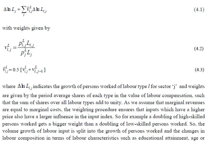 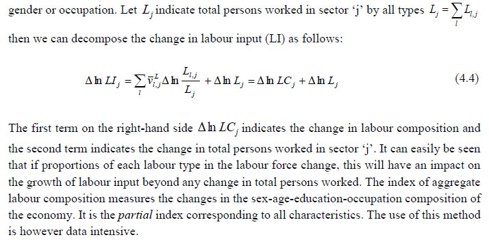 There is a second approach to the measurement of skill levels. The procedure is to use a simple index of educational attainment to adjust for skill differences. So improvement in educational attainment is adjusted by incorporating average years of schooling as the proxy for skill levels. For example, an index of the form: L* = easL assumes that each year of schoolings, raises the average worker’s productivity by a constant percentage, ‘a’. Such studies have been carried out for different time periods and for a large number of countries around the world, typically finding a return to each additional year of education in the range of 7 to 12 percent (BCV, 2007). Most of the recent indices of composition of labour input are based on the methodology of Jorgenson, Gollop, and Fraumeni (JGF) (1987) and uses the Törnqvist translog index. However, this methodology requires large volume of data. Using this methodology Aggarwal (2004) estimated labour composition for the Indian manufacturing labour force. There are however, lot of disagreements on the use of this methodology in the Indian context, as it assumes the existence of perfectly competitive labour markets where wage rate is the indicator of a person’s marginal productivity. The analysts argue that the observed wage differences may reflect factors other than productivity differences, such as age or gender. Its use is also questioned because data for large segment of Indian labour force- the self -employed is not available. Since the Indian labour market is still not very competitive and there are data weaknesses, therefore the researchers in India have generally avoided applying the JGF methodology. For this reason, most Indian researchers have avoided to account for the differences in age and gender characteristics. However, to account for educational differences they have preferred to exercise either of the two choices- one to use Barrow and Lee (1993) methodology and presume a constant rate of return for education (BCV, 2007) or second is to use the limited information available on wages for few rounds and only for casual and regular employees (Sivasubramonian, 2004) to determine the weights of different types of persons. Bosworth and Collins (2008) assumed a constant annual return of 7 percent for each additional year of education irrespective of the level of education. The problem with the assumption of uniform returns for each year is that it ignores all variations- across levels of education, over gender, over age groups, over industries, etc. and only includes education. It is thus not able to capture the impact of change in gender composition, age composition (a proxy for experience) and industry composition. The present version of the manual and report now has included two of these characteristics. So a Grand labour composition index, an Education, and an Age labour composition index have been estimated based on JGF methodology using suitable data. The gender characteristics is avoided as Indian females still have very low level of education in general and higher education in particular, especially among the middle and senior age group. Therefore, either no data is available or there are very few sample observations for many such cells with cross classification of education, age and industry. The data for the survey years on total number of persons employed by each industry is taken from the current employment series. The data on employment is essentially derived from the unit level record data of National Sample Survey (NSS) which is made available by NSSO in the form of CD-ROMS for the five Quinquennial rounds beginning from 38th. We estimated the number of employed persons according to UPSS as follows:
For extrapolation backward to 1980-81 to 1982-83, the interpolation of the broad industrial classification of 32nd round and 38th round is used. So the estimates from 32nd round are mainly used as control numbers. For the construction of the three labour composition indices we require data on employment and earnings by education, and age for the broad sectors and for each of the 27 industries. We distinguish three types of educational categories for broad sectors and three types of educational categories for each of 27 industries because of large data requirement at disaggregate level. The three education categories used are ‘up to primary’, ‘above primary to higher secondary’, and ‘above higher secondary’. The three age groups used are 14-30, 30-49, above 49 years. Table 4.1 below summarizes all this. Therefore the following additional steps have also been performed: i) The first step involves computing the proportions of the distribution of persons employed by the three age and educational groups for the selected major rounds. ii) These proportions are then applied to the number of employed persons in different industries to obtain the distribution of persons by age and education groups. iii) The earnings data is estimated from NSSO which relates it mainly to regular and casual persons employed. It may however be mentioned that even for these two groups, for a large number of persons employed, the wages are either missing or given as zero. iv) For earnings of self-employed persons19, two approaches have been adopted. Firstly, a Mincer wage equation has been estimated and the sample selection bias is corrected for by using the Heckman’s20 two step procedure. The function has been applied to the earnings of casual and regular employees where the earnings have been regressed on the dummies of age, gender, education, location, marital status, social exclusion and industry. The identification factors used in the first stage are age, gender, and marital status, type of household/size of household. The corresponding earnings of the self-employed are obtained as the predicted value with similar traits. The average wages per day are then computed for persons employed of different type of employment, i.e. self-employed, regular and casual combined together; whose wages are more than zero. Secondly, earnings of self-employed have also been estimated from the monthly consumption expenditure of these households. In this, first the total monthly consumption expenditure is divided by the number of employed persons in the household to get total monthly consumption expenditure per employed person. Then the ratio of wage earnings to total monthly consumption expenditure per employed person has been calculated for each industry by UPSS status for the selected rounds. Assuming the consumption earnings ratio to be same for casual and self-employed persons, the ratio for casual labour is used for self-employed persons and this ratio is multiplied to the total monthly consumption expenditure per self-employed person so as to get the earnings of the self-employed persons. However, if the earnings thus obtained are higher than the earnings obtained from Mincer equation, then the latter are used. So the lower of the two- earnings -obtained from Mincer equation or the earnings based on consumption expenditure, are taken to be the earnings of the self-employed persons. Once the above steps are taken to find out the age and educational distribution of all employed persons in all the five rounds and their corresponding wages, the computation of the grand labour composition index; the age composition index and the education composition index are carried based on the JGF (1987) methodology with 1980-81 equal to 100. The indices are estimated for total persons working in 27 different industries in India for the 38th, 50th, 55th, 61st, and 68throunds of NSSO with 1983 (38th round) equal to 100 so as to assess the temporal changes in labour skill. Since the series required is from 1980-81, we have extrapolated it backwards from 1983 to 1980-81. The next phase of this project aims to update the series and perform some robustness checks of the current employment series with the help of the next round of EUS data, which is expected in 2018-19 and bring out policy implications from the employment trends. Appendix C: Definitions of Employment in NSSO employment & unemployment surveys The surveys of NSSO on employment and unemployment (EUS) aim to measure the extent of ‘employment’ and ‘unemployment’ in quantitative terms disaggregated by various household and population characteristics following the three reference periods of (i) one year, (ii) one week, and (iii) each day of the week. Based on these three reference periods three different measures, termed as usual status, current weekly status, and the current daily status, are arrived at. While all these three approaches are used for collection of data on employment and unemployment in the quinquennial surveys, the first two approaches only are used for the purpose in the annual surveys. Usual principal status: In NSS 27th round, the usual principal activity category of the persons was determined by considering the normal working pattern, i.e., the activity pursued by them over a long period in the past and which was likely to continue in the future. For the identification of the usual principal status of an individual based on the major time criterion, in NSS 27th, 32nd, 38th, 43rd rounds, a trichotomous classification of the population was followed, that is, a person was classified into one of the three broad groups ‘employed’, ‘unemployed’ and ‘out of labour force’ based on the major time criterion. From NSS 50th round onwards, the procedure was changed and the prescribed procedure was a two stage dichotomous one which involved a classification into ‘labour force’ and ‘out labour force’ in the first stage, and thereafter, the labour force into ‘employed’ and ‘unemployed’ in the second stage. Usual subsidiary status: In the usual status approach, besides principal status, information in respect of subsidiary economic status of an individual was collected in all employment and unemployment surveys. For deciding the subsidiary economic status of an individual, no minimum number of days of work during the last 365 days was mentioned prior to NSS 61st round. In NSS 61st round, a minimum of 30 days of work, among other things, during the last 365 days, was considered necessary for classification as usual subsidiary economic activity of an individual. Current weekly status: It is important to note at the beginning that in the EUS of NSSO, a person is considered as worker if he/she has performed any economic activity at least for one hour on any day of the reference week and uses the priority criteria in assigning work activity status. This definition is consistent with the ILO convention and used by most of the countries in the world for their labour force surveys. In NSSO, prior to NSS 50th round and in all the annual surveys till NSS 59th round, data on employment and unemployment in the CWS approach was collected by putting a single-shot question ‘whether worked for at least one hour on any day during the last 7 days preceding the date of survey’. The information so collected was used to determine the CWS of the individuals. This procedure was criticized for being not able to identify the entire workforce, particularly among the women. It was then decided to derive the CWS of a person from the time disposition of the household members for the 7 days preceding the date of survey. The procedure was used for the first time in NSS 50th round. It is seen that the change in the method of determining the current weekly activity had resulted in increasing the WPR in current weekly status approach - more so for the females in both rural and urban areas than for males. The trend observed in NSS 50th round in respect of the WPR according to CWS suggested continuing with the procedure for data collection in CWS in NSS 55th and NSS 61st rounds. Current Daily Status Current Daily Status (CDS) rates are used for studying intensity of work. These are computed on the basis of the information on employment and unemployment recorded for the 14 half days of the reference week. The employment statuses during the seven days are recorded in terms of half or full intensities. An hour or more but less than four hours is taken as half intensity and four hours or more is taken as full intensity. An advantage of this approach was that it was based on more complete information; it embodied the time utilisation, and did not accord priority to labour force over outside the labour force or work over unemployment, except in marginal cases. A disadvantage was that it related to person-days, not persons. Hence it had to be used with some caution.
Chapter 5: Capital Input Series at the Industry Level This chapter outlines the methodology employed to estimate capital services for the 27 industries in the India KLEMS database version 2017. Following an overview of the theoretical method developed by Jorgenson and Griliches (1967), and outlined in Jorgenson, Gollop and Fraumeni, (JGF, 1987), the Chapter discusses the specific empirical approaches we follow to implement these methods within the constraints of data availability for Indian industries. For the measurement of capital services we need capital stock estimates for detailed asset types and the shares of each of these assets in total capital remuneration. Using the Törnqvist approximation to the continuous Divisia index under the assumption of instantaneous adjustability of capital, aggregate capital services growth rate is derived as a weighted growth rate of individual capital assets, the weights being the compensation shares of each asset, i.e. 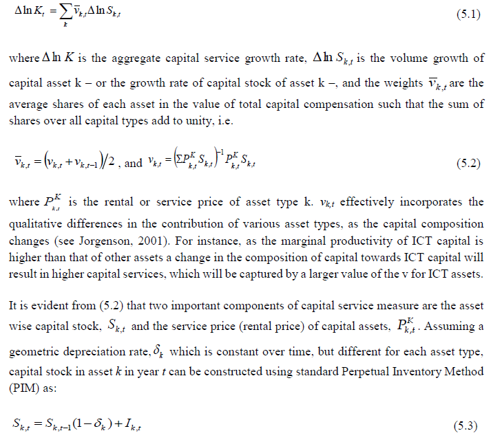 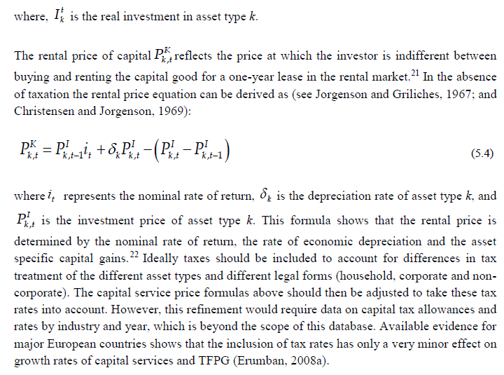 Since our measure of capital input takes account of asset heterogeneity, it was essential to obtain investment data by asset type. We distinguish between 3 different asset types – construction, transport equipment, machinery (includes ICT and non-ICT machinery).23 We exploit multiple sources of information for the construction of our database on capital services. This includes the National Accounts Statistics (NAS) that provide information on broad sectors of the economy, the Annual Survey of Industries (ASI) covering the organized manufacturing sector, the National Sample Survey Organizations (NSSO) rounds for unorganized manufacturing and Input-Output tables. Even though we use multiple sources of data, our final estimates are fully consistent with the aggregate data obtained from the NAS. In addition, our approach to capital measurement is consistent with international practices such as the EU KLEMS24, which ensures the possibility of international comparisons. In what follows we discuss the various sources of data for asset wise investment and the construction of the relevant variables, in detail. (a) Asset-wise investment for broad sectors of the economy Industry-level estimates of capital input require detailed asset-by-industry investment matrices. NAS provides information on aggregate capital formation by industry of use for 9 broad sectors, which, nevertheless, was not sufficient for our purpose. Therefore, we have collected more detailed data on assets and industries from the CSO.25 This is the data underlying the published aggregate gross fixed capital formation by the broad industry groups, separately for public and private sectors. For those sectors for which the investment matrices were not available from CSO, we gather information from other sources (e.g. ASI for organized manufacturing and NSSO surveys for unorganized manufacturing) and benchmark it to the aggregate investment series from the National Accounts. The data used in the current version of the India KLEMS is based on the revised NAS with 2011-2012 base, and is available only since 2012. Therefore, for earlier years, we extrapolate the series using growth rates from previous version of the data. However, there were slight differences between the industry groups available in the current release of the data and the previous ones (see Table 5.1), which required some matching of sectors before combining the two series. Table 5.2 provides an overview of asset types available in NAS and their corresponding asset types used in our study.
Total investment in each asset category is calculated as the sum of private and public sector investment in each asset. Investment in transport equipment is not available separately for private sector. We tried several approaches to impute the private sector transport equipment data. The first was to use the share of transport equipment in non-departmental enterprises. More specifically, we apply the non-departmental enterprise transport equipment to machinery & equipment (including transport equipment) ratio to machinery & equipment in private sector for each industry to obtain industry wise transport equipment for private sector. We take non-departmental enterprise only, rather than the entire public sector, as it may be more realistic as it consists of public sector companies and statutory corporations, excluding administrative sector. However, the sum of industry estimates generated by this approach was not consistent with the reported aggregate private sector transport equipment. Therefore, we take a second step here, which is to use the industry distribution from this series and apply it to the published total private sector transport equipment data. The estimated transport equipment is then subtracted from each industry’s total machinery & transport equipment data, to obtain machinery in private sector as a residual. However, this approach generates many negative numbers in transport equipment in private sector, particularly in transport services. Therefore, we follow a third approach, which is what we finally use in the database. We first distribute the NAS total machinery in the private sector using the industry distribution of machinery and transport equipment. These estimates are then subtracted from each industry’s total machinery & transport equipment data to obtain the transport equipment investment in the private sector industries. (b) Asset-wise investment for non-NAS sectors NAS provides data only for 9 broad sectors, while we have 27 industries, which necessitated further splitting of some of the NAS sectors. This includes aggregate manufacturing (registered and unregistered separately) with 13 sub sectors; other services into 4 sub sectors; and real estate activities and business services into 2 sub sectors. The manufacturing sector investment data was disaggregated into 13 subsectors at the 2 digit level of NIC 1998 using ASI and NSSO data, which will be discussed in detail subsequently. Investment series in service sector has been split into sub sectors using two alternative approaches–value added shares, and capital/labour ratio in the higher aggregate industry. However, the final data used are based on value added shares, as a sensitivity analysis did not show a significant difference between the two. In order to split the aggregate capital formation in organized manufacturing sector into 13 study sectors, we use the Annual Survey of Industries. However, the published data does not provide any asset wise investment information; it consists of only the aggregate capital formation or the book value of fixed capital. Most studies in the past have measured gross investment as the difference between book value of asset in period t and in period t-1 and add depreciation in period t to that. This approach has the deficiency of comparing two different samples reported in two different years, where the number of firms/factories might be different. In particular, while using this approach at industry level, for detailed asset categories, it might generate massive negative investment. We follow an alternative approach, following ASI’s definition of gross fixed capital formation (GFCF). ASI defines GFCF as actual additions (newly purchased, second hand and own construction) minus deductions plus depreciation adjustment for discarded assets during the year. This approach is based on a single year’s sample and helps to avoid potential huge negative investment series, and is also consistent with published ASI GFCF series. The yearly detailed volumes beginning 1964-65 were used to derive the gross fixed capital formation by asset type directly. For the years 1964-1978, the relevant data are obtained from published detailed volumes. For the period, 1983-84 to 2004-05 ASI has generated detailed tables from Block C of ASI schedule that contain data on fixed assets. Data for missing years are interpolated using the changes in investment using book value method. Table 5.3 provides an overview of the asset categories available in ASI, and the relevant asset categories in our study to which they are attributed. Though ASI provides investment in land, for reasons of NAS consistency we exclude it from our database. Once investment in each of these assets and industries are generated using ASI data, we apply this industry-asset distribution to the published aggregate NAS GFCF series for organized manufacturing sector. It may also be noted that from 1960-61 to 1971-72, ASI data are for the census sector and from 1973-74 on wards they are for the factory sector. In order to make these two series comparable over years, we convert the data prior to 1972 to factory sector using the factory/census ratio in 1973. Thus, after these adjustments, we obtain investment data for 13 manufacturing sectors, by asset types, consistent with the NAS aggregate. The data required for creating the gross investment series for the 13 sectors of the unorganized manufacturing sector are obtained from various rounds of NSSO surveys on unorganized manufacturing. We use 6 rounds of NSSO surveys that cover the period 1989-2016. These are 45th round (1989-90), 51st round (1994-94), 56th round (2000-01), 62nd round (2005-06), 67th round (2010-11) and 73rd round (2015-16). Unit level data has been aggregated to 13 industries using the appropriate concordance tables. NSSO provides net addition to owned assets during the reference year within the block of fixed assets, and we use this as a measure of our investment. Asset classification in NSSO has changed over various rounds, and therefore, we have tried to match these with our classification as shown in Table 5.4. The investment series arrived at for four rounds were interpolated to obtain the annual time series of unorganized gross fixed capital formation by asset type. As in the case of registered sector, once the investment by asset types across industries are constructed, the asset-industry distribution is applied to the published NAS aggregate GFCF in unregistered manufacturing to obtain NAS consistent GFCF by asset type and industries. (c) Investment Prices by Asset Types In order to compute asset wise capital stock using PIM (equation 5.3) and rental price (equation 5.4), we require asset wise investment price deflators. Since CSO has provided us with investment data by industries and assets both in current and constant prices, we could derive the price deflators with base 2011-2012. For years before 2011, prices were spliced using 2004-2005 base investment deflators. These deflators are directly used for all the three asset categories we have. (d) Initial Stock, Depreciation Rates and Rate of Return As is evident from equations 5.1 to 5.4, our estimates of capital input require time-series data on asset wise capital stock. Capital stock has been constructed using perpetual inventory method (PIM), where the capital stock (S) is defined as a weighted sum of past investments with weights given by the relative efficiencies of capital goods at different ages, which requires data on current investment by asset types, investment prices by asset types and depreciation rate. Also, for the practical implementation of PIM to estimate asset wise capital stock, we require an estimate of initial benchmark stock (see Erumban, 2008b for an in-depth discussion on this issue). NAS provides estimates of net capital stock since 1950 for all the broad sectors in its Statement 17: Net Fixed Capital Stock by industry of use. We take the NAS estimate of real net capital stock in 1950 (in 1999-2000 prices) as our benchmark stock for all non-manufacturing sectors, and for manufacturing sectors the same is taken for the year 1964.27 However, since the NAS estimate is available only for broad sectors and for aggregate capital, we use our industry-asset distribution of GFCF in order to create net fixed capital stock estimates by asset type for all the 27 sectors. NAS also provides detailed tables on assumed life of assets used for computing capital stock, for private units, administrative units as well as departmental and non-departmental units by asset types.28 We use these estimates of lifetime to derive appropriate depreciation rates for non-ICT assets, using a double declining balance rate. We assume 80 years of lifetime for buildings, 20 years for transport equipment, and 25 years for machinery and equipment. The final depreciation rates used in the study are given in Table 5.5 by asset type. Subsequently, we build our capital stock series by asset types for all the 27 industries using our GFCF series from 1950 (1964) onwards for the non-manufacturing (manufacturing) sectors. Our measure of capital input is arrived using equation (5.1), for which we also require estimates of rental prices (see equation 5.4). Assuming that the flow of capital services is proportional to the capital stock at individual asset level, aggregate capital flows can be obtained using a translog quantity index by weighting growth in the stock of each asset by the average shares of each asset in the value of capital compensation, as in (5.1). The rate of return (i) in equation (5.4) represents the opportunity cost of capital, and can be measured either as internal (or ex post) rate of return, or as an external (ex ante) rate of return.29 This issue will be addressed in the further revisions of the data. The present version of the database uses an external rate of return, proxied by average of return on government securities and prime lending rate obtained from the Reserve Bank of India30. Therefore, we use a real rate, which is net of capital gain. Hence, the capital gain component in equation (5.4) is excluded while estimating rental price using external rate of return, obtaining  Where i* is the real rate of return, nominal interest rate adjusted for CPI inflation rate. Chapter 6: Intermediate Input Series at the Industry Level In this section we describe the basic approach we have used to derive the volume series of Intermediate Inputs namely –Energy input (E), Material input (M) and services input (S). This breakdown of intermediate inputs can be used for extending the growth accounting exercises, but also convey interesting information about changing pattern in intermediate consumption (see e.g. JHS 2005, chapter 4) The methodology for measuring industry output, intermediate inputs and value added was developed by Jorgenson, Gallop and Fraumeni (1987) and extended by Jorgenson (1990 a). The cornerstone of this approach is a time series of input output (IO) tables which gives the flows of all commodities in the economy, as well as payments to primary factors. Every commodity is accounted for, whether produced by a domestic source or imported, and every use is noted, whether purchased by an industry or by a final demand element. All payments to factors of production i.e. labour and capital is accounted for so that all income elements of GDP are included. The methodology of constructing time series on energy, material and services inputs for the European economy has been elucidated in Timmer et al. (2010, Chapter 3). Following a similar approach as explained in Jorgenson et al. (2005, Chapter 4) and Timmer et al. (2010, Chapter 3), the time series on intermediate inputs for the India KLEMS project have been constructed. Definition of EMS: As in EU KLEMS, this study identifies three main categories of Intermediate inputs. They are classified as follows:
Intermediate Inputs are broken down into energy, material and services, based on input output transaction tables using a standard NIC product classification. The following five energy types (and products) have been classified as the Energy input.
The following fourteen input items have been classified as the Service input
All other intermediate inputs barring the above mentioned nineteen inputs are classified as material input. The key building block for constructing time series on Intermediate Inputs at current prices, as explained in Jorgenson et al. (2005, Chapter 4), is the input-output transaction tables, that is, the inter industry transaction tables that provide a description of which industries produce each product and which industries use them. The input-output table gives the inter-industry transactions in value terms at factor cost presented in the form of commodity x industry matrix where the columns represent the industries and the rows as group of commodities, which are the principal products of the corresponding industries. Each row of the matrix shows in the relevant columns, the deliveries of the total output of the commodities to the different industries for intermediate consumption and final use. The entries read down industry columns give the commodity inputs of raw-materials and services, which are used to produce outputs of particular industries. The column entries at the bottom of the table give net indirect taxes (NIT) (indirect taxes – subsidies) on the inputs and the primary inputs (income from use of labour and capital), i.e., Gross Value Added (GVA). As the IOTT is in the form of commodity x industry matrix, the row totals do not tally with the column totals. The difference between each column and the corresponding row totals is due to the inclusion of the secondary products, which appear particularly in the case of manufacturing industries. This is so because by-products are also manufactured by industries in addition to their main products. Thus, while determining the entries in the rows, a by-product of an industry is transferred to the sector (commodity row), whose principal product is the same as the by-product under reference. The columns, however, show the total of principal products and by-products of each industry. All the entries in the IOTT are at factor cost, i.e. excluding trade and transport charges and NIT. The Input Flow Matrix at factor cost, published by CSO, for 1978 is a 60 x 60 matrix. The absorption matrices for 1983, 1989, 1993 and 1998 have 115 sectors. However a detailed 130 sector absorption (commodity x industry) matrix for the Indian economy has been published from 2003-04 onwards. The scheme of sector classification adopted in supply use table 2012-13, IOTT 2007-08 and IOTT 2003-04 vis-à-vis , IOTT 1983-84, IOTT 1989-90, IOTT 1993-94 and 1998-99 has undergone significant change with the disaggregation of some of the sectors, which have become significant in early 2000s.
The methodology for computation of Intermediate Input Series for 27 Industries from 1980-2014 at current and constant prices is explained in steps. Step 1: Concordance is done between IOTT and study industries
Step 2: Obtaining estimates for Material, Energy and Service Inputs for 27 Industries, in benchmark years
Thus, for each of the benchmark year, estimates are obtained for Material, Energy and Service Inputs that has been used to produce Gross output in the 27 different India KLEMS Industries. Step 3: Projecting a time series (1980 to 2015) of proportions of Material, Energy and Service Inputs in Total Intermediate Inputs for each of the 27 industries
There exist some abnormal fluctuation in the proportions of Material Inputs, Energy Inputs, and Service Inputs in Total Intermediate Inputs for benchmark years. In that case we drop that specific benchmark proportion and linearly interpolate of the adjacent benchmark proportions to estimate proportion for intervening years. For the industry group ‘Coke, Refined Petroleum and Nuclear Fuel’, we estimated proportions of Material Inputs, Energy Inputs, and Service Inputs in Total Intermediate Inputs from ASI data instead of Input Output Transaction Table. This has been done because the relevant proportions differed significantly between the input-out tables and ASI, and the latter is believed to be making a more correct assessment of energy inputs used in the Coke and Petroleum products industry. For example, coal consumed in the Coke industry is the taken primarily as material rather than energy. From IOTT it is difficult to estimate how much of coal consumption is for energy purposes and how much as material input, where ASI provides details information about energy consumption by energy inputs like: coal, electricity, petroleum and others including natural gas. Step 4: Consistency with NAS The projection of intermediate input vector, using IOTT in Step 3 needs to be consistent with the estimated output from NAS.
1. For Benchmark years: Ratio of Total Intermediate inputs from NAS to that from IOTT is adjusted proportionately to the absolute value of Energy Inputs/Material Inputs/Service Inputs obtained from IOTT. 2. For Intervening Years: The interpolated proportions of Energy Inputs, Material Inputs and Services Inputs obtained from IOTT, is applied directly to the total intermediate inputs from NAS to get each inputs share. Two examples have been given below for the Construction sector: In the examples above, we can see that the total value of intermediate input exactly matches the gap between Gross output and Value added. Similar adjustments have been made to construct the input series for all the other 27 study industries from 1980-2015. For every benchmark year where IOTT is available adjustment ‘A’ has been done. For every non-benchmark year, where IOTT is not available and an intermediate input vector has been projected, adjustment ‘B’ has been done to generate the comprehensive time series of Intermediate inputs consistent with the official National Accounts. Steps 1-4: This gives a time series of Material, Energy, and Service Inputs for 27 study Industries from 1980 to 2015 at current prices. Steps 5 and 6 below, explain the methodology for computation of Intermediate Input Series for 27 study Industries from 1980-2015 at constant price. The approach followed here is to first form the aggregates of materials, energy and services at current price for each study industry from the benchmark Input Output tables and then develop deflators of Materials, Energy and Service Inputs for each of the 27 study Industries separately. Step 5: Constructing Deflators of Materials, Energy and Service Inputs for 27 study Industries separately
Step 6: Computing Time Series on Intermediate Input for 27 study Industries from 1980-2014, Constant prices
Thus we have a time series of Material, Energy and Service Inputs for 27 study Industries at constant prices. Firstly, Input Output transaction tables are generally available on a five year interval period and this necessitates interpolation and assumption of constant shares in some cases, to construct the entire time series of EMS from 1980 to 2015. Secondly, unlike studies using detailed survey data, we have to assume that all buyers pay the same price for each commodity because there is no information about price divergences. Thirdly, The estimated time series of Intermediate Inputs at constant price will not be consistent with the intermediate input of NAS at constant price i.e. the deflated value of intermediate input cannot match the gap between value added and gross output at constant price from NAS. This is because; NAS uses a single deflation method to estimate Gross Value Added and Gross Output at constant price. ‘However, only for one sector – Agriculture, the Gross Output and Gross Value Added, estimated by NAS is double deflated. Therefore only for the Agriculture sector the deflated value of intermediate input will exactly match the gap between value added and gross output at constant price. Fourthly, there has been some confusion in the literature on the price concept to be used for intermediate inputs. It is generally acknowledged that the intermediate input weights should be measured from the user’s point of view, i.e. reflect the marginal cost paid by the user. Most studies maintain that purchaser’s price should be used. These prices include net taxes on commodities paid by the user and include margins on trade and transportation (see, for example OECD 2001). However when trade and transportation services are included as separate intermediate inputs, margins paid on other products should also be allocated to these services. Ideally a distinction should be made between the intermediate product valued at purchaser’s price minus margins and the trade and transportation services valued at margins. This is the approach taken in Jorgenson, Gollop and Fraumeni (1987). and in Jorgenson et al. (2005). However Timmer et al. (2010, Chapter 3) explains that for the EU KLEMS database, intermediate inputs have been valued at purchaser’s price owing to unavailability of necessary data. Because of the use of purchaser’s price concept the shares of services in intermediate inputs do not include trade and transportation margins. Similarly in practice for the database, the time series of Intermediate Input constructed is at purchaser’s price i.e. it implicitly takes into account the net indirect taxes. The distribution of this net indirect tax between Material, Energy and Services has not been possible because of unavailability of a time series of tax matrix from 1980 to 2015. Chapter 7: Factor Income Share Series at the Industry Level The distribution of income between capital , labour and intermediate inputs, is an important element in growth accounting because income shares, under conditions of competitive markets, can be used to measure the contributions each factor makes towards output growth. 7.1 Methodology for Measuring Labour Income Share Series Under the assumption of constant returns to scale with two factors of production i.e., labour and capital, the sum of the labour income share and capital income share is 1. The labour income share is defined as the ratio of labour income to GVA. Capital income share is accordingly obtained as one minus labour income share. There are no published data on factor income shares in Indian economy at a detailed disaggregate level. National Accounts Statistics (NAS) of the CSO publishes the NDP series comprising of compensation of employees (CE), operating surplus (OS) and mixed income (MI) for the NAS industries. The income of the self-employed persons, i.e. mixed income (MI) is not separated into the labour component and capital component of the income. Therefore, to compute the labour income share out of value added, one has to take the sum of the compensation of employees and that part of the mixed income which are wages for labour. The computation of labour income share for the 27 study industries involves two steps. First, estimates of CE, OS and MI have to be obtained for each of the 27 study industries from the NAS data which are available only for the NAS sectors (see Table 7.1). Second, the estimate of mixed income has to be split into labour income and capital income for each industry for each year (except for those industries for which the reported mixed income is zero, for instance, public administration). Basis data sources used for the computation of labour income share are NAS, ASI and unit level data of survey of unorganized manufacturing enterprises. These data sources are used to obtain estimates of CE, OS and MI for each of the 27 study industries. For splitting the labour and non-labour components out of the mixed income of self-employed, the unit level data of NSS employment-unemployment survey are used along with the estimates of CE, OS and Mi basically obtained from the NAS. a) Construction of Labour Income Share Series in Gross Value Added The estimation of labour income share for the 27 study industries has been done in two steps, as discussed below. Step 1: Estimation of CE, OS and MI for the 27 study Industries For some industries under study, for instance (i) Agriculture, forestry & logging and fishing, (ii) Mining & Quarrying, (iii) Electricity, gas and water supply and (iv) Construction, the required data are readily available from NAS. For others, the estimates available in NAS have to be distributed across the study industries. In certain cases, the estimates of CE, OS and MI for a particular NAS sector have been distributed across constituent study industries proportionately in accordance with the gross value added in those industries. Estimate of factor incomes for ‘other services’ in NAS , for instance, has been split into estimates for (i) Education, (ii) Health and Social Work, and (iii) Other Community, Social and Personal Services including Renting of machinery and business services, and Private Household with Employed Persons. NAS provides estimates of factor incomes for registered manufacturing and unregistered manufacturing, but not for individual manufacturing industries. The NAS estimates of factor incomes for registered manufacturing have to be split into various manufacturing industries considered in the study (13 in number) using ASI data. The reported CE in NAS for registered manufacturing has been distributed into those 13 industries in proportion to the reported ASI data on emoluments for various industries. In a similar way, using ASI data, the estimate of OS for registered manufacturing has been distributed. Emoluments are subtracted from gross value added for various industries yielding capital income. The share of different industries in aggregate capital income of organized manufacturing indicated by the ASI data is used to split the estimate of OS for registered manufacturing reported in the NAS. The methodology applied for unregistered manufacturing is similar. The published results and unit level data of survey of unorganized manufacturing industries have been used for this purpose. The estimates of wage payments (to hired workers) in different industries have been used to split (proportionately) the estimate of CE in the NAS for aggregate unregistered manufacturing. The estimated wage payment is subtracted from the estimated value added to obtain an estimate of capital income and mixed income of the self employed in various unorganized manufacturing industries. The estimate of MI provided in NAS for unregistered manufacturing has then been proportionately distributed across industries using the estimate of capital income and mixed income of the self-employed in various industries that could be formed on the basis of published results and unit level data of survey of unorganized manufacturing industries. Unlike the ASI data for organized manufacturing, the data for unorganized manufacturing enterprises are available for only select years. The proportions mentioned above could therefore be computed only for those select years (data for five rounds have been used; these are for 45th round (1989-90), 51st round (1994-95), 56th round (2000-01), 62nd round (2005-06), 67th round (2010-11) and 73rd round (2015-16)). It has accordingly been necessary to resort to interpolation/ extrapolation to obtain the relevant proportions for other years. Step 2: Splitting of MI into Labour Income and Capital Income As explained above, the income share of labour is computed as:  The derivation of the GVA series for different industries has been briefly explained in Chapter 2. The derivation of CE and MI series has been explained in step I above. Therefore, only the estimation method of ƞ needs to be described. The estimation of ƞ has been done with the help of NSS survey based estimates of employment of different categories of workers (number of persons and days of work) and wage rates (which has been described briefly in chapter 4) coupled with estimates of MI, basically obtained from the NAS. Two approaches have been taken to get an estimate of ƞ, and the labour income share series for different industries finally adopted in the study makes use of an average of the estimates of ƞ obtained by the two approaches. In the first approach, an estimate of labour income of self-employed workers has been made for each study industry for five years, 1983-84, 1987-88, 1993-94, 1999-00, 2004-05, 2009-10, 2011-12 and 2015-16 on the basis of the estimated number of self-employed, wage rate of self-employed and the number of days of work per week. The industry-wise estimates of number of self-employed, wage rate of self-employed and the number of days of work per week have been made from unit records of NSS employment-unemployment survey (major rounds), as explained in chapter 4 above. The estimates of the number of self-employed, wage rate of self-employed and the number of days of work per week provide an estimate of the annul labour income of self-employed workers which is divided by the mixed income of self-employed (derived from NAS) to get an estimate of ƞ. For five industries, the ratio in question has been computed and applied. For the other 22 industries, the ratio in question has been computed after clubbing the industries into 11 industry groups.31 In the latter case, a common ratio computed for group of industries has then been applied to constituent industries. The list of industries or industry groups for which ƞ has been estimated is given in table 7.2. In the second approach, the NSS data are used to compute the following ratio: the ratio of labour income of self-employed workers to the labour income of regular and casual workers. Let this be denoted by θ. Then, the estimate of CE provided in the NAS is multiplied by θ to obtain an estimate of the labour income component out of the MI reported in the NAS. The labour component of MI divided by total MI gives an estimate of ƞ. In case the estimated labour component of MI exceeds the estimate of MI, the estimate of ƞ has been taken as unity. Examining the estimates obtained by the first approach, it was found that the estimated labour income share out of mixed income varied significantly among the estimates for the seven years for which the ratio in question has been estimated. The estimates of ƞ obtained by the second approach has the problem that in a number of cases, the estimated labour component of MI exceeds the estimate of MI given in the NAS, and therefore ƞ is taken as one. The method finally adopted is as follows: (a) The average value of ƞ has been computed for each industry or industry group by taking the estimates for the years 1983-84, 1987-88, 1993-94, 1999-00, 2004-05, 2009-10, 2011-12 and 2015-16. This has been done separately for the estimates based on approach-1 and those based on approach-2. (b) The estimates of ƞ obtained for each industry or industry group by the two approaches have then been averaged. (c) Having obtained an estimate of ƞ, equation 6.1 given above has been applied to compute the labour income share. b) Construction of Factor Income Share Series in Gross output The income share of labour, capital and intermediate inputs in Gross output has been computed using the following steps:
The splitting of unorganized sector factor incomes into individual industries has been done using unorganized survey results. The proportions computed for 1983-84 has been applied for the period 1980-81 to 1983-84. While there were surveys of unorganized manufacturing enterprises in 1978-79 and 1984-85, the survey results have not been used for estimation of factor incomes in different industries of the unorganized manufacturing sector. At attempt will be made to use survey data for the years 1978-79 and 1984-85 rather than applying the proportions computed for 1989-90 to factor income data for earlier years. In case of KLEMS data series, we have used CE, OS and MI data from NAS. As NAS provides information on CE and OS for aggregate registered manufacturing. So we distribute it among 13 registered manufacturing industries using ASI information. Similarly for unorganized manufacturing we have information on CE and MI. so we distribute it using NSSO information. And then add up the registered and unregistered portion to get overall manufacturing CE, OS and MI. In case of organized and unorganized manufacturing data set, we use Emoluments/GVA from ASI as labour income share for organized manufacturing industries. And Emoluments/GVA for NDME+DME as labour income share for unorganized manufacturing. Chapter 8: Growth Accounting Methodology This chapter deals with the methodology of measurement of total factor productivity (TFP) growth for individual industries in the KLEMS framework and the aggregation from industry level productivity measures to measures for broad sectors and the economy as a whole. The methodology of analysis of sources of gross output growth at the individual industry level and sources of GVA (Gross Value Added) or GDP growth at the broad sector level and economy level will also be presented in this chapter 8.1 Methodology for Measuring Productivity Growth at the Industry level The production function Our measurement of TFP growth for different industries of the Indian economy is based on a gross output production function for each industry j: Y is industry gross output, L is labour input, K is capital input and E, M and S are intermediate inputs-namely energy, material and services and T is an indicator of technology for industry j. All variables are indexed by time (t subscript is suppressed). There are several things to note about the production function- (1) all variables are aggregates of many components that have been discussed in the earlier report/chapters; (2) we assume that the industry production function is separable in these aggregates; (3) time (indicator of technology) enters the production function symmetrically and directly with inputs. An important feature of the gross output approach is the explicit role of intermediate inputs. In our study, we have considered three intermediate inputs - energy, material and services and this is important as we may find that intermediate inputs are the primary component of some industries outputs.32 Failure to quantify intermediate inputs leads us to miss both the role of key industries that produce intermediate inputs and the importance of intermediate inputs for the industries that use them. In order to estimate the production function at constant prices, the industry level price data is used for output, capital, labour and intermediate inputs, e.g., PYj; PLj, PKj; PEj. PMj, PSj. We assume that all industries face the same input price. The industry price of an input varies across industries due to compositional effects as industries expend different shares of their investment on each type of asset. The same is true for all inputs. Total Factor Productivity 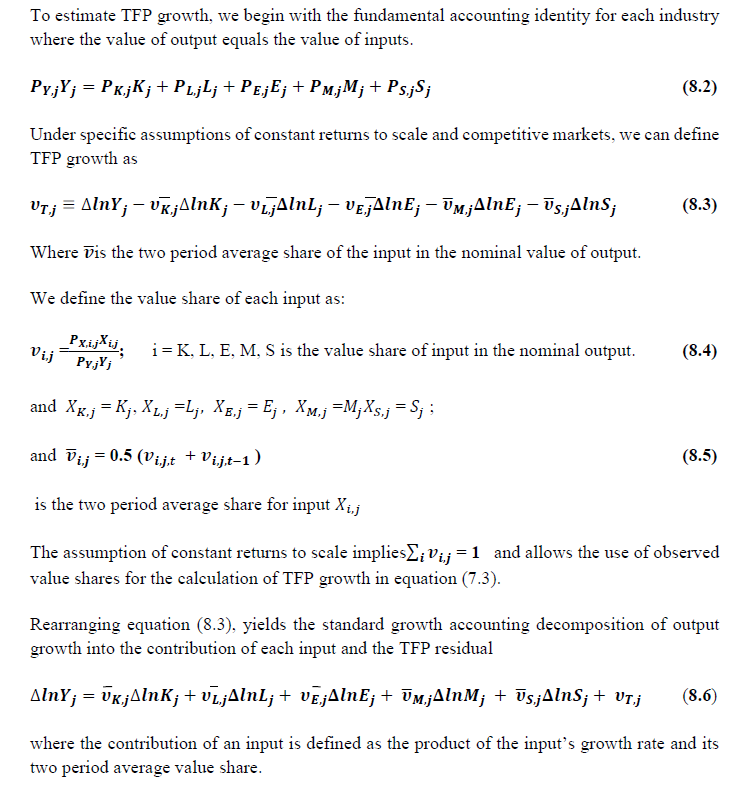 We can further decompose the contribution of each input into a quantity and quality component. As discussed earlier, the quality component represents substitution between H components, while the quantity component represents the increases in each detailed input. Our extended decomposition of the sources of output growth is 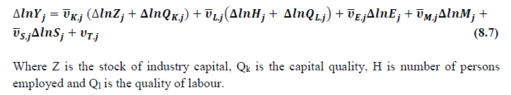 8.2 Methodology for Aggregation across Industries In the analysis presented in the above section, gross value of output (GVO) is taken as the measure of output of an industry and TFP growth was estimated using the gross output function framework in which capital, labour, materials, energy and services are taken as five inputs (in the case of agriculture, land was included among inputs). The Törnqvist index is applied to estimate TFP growth for each year during 1980-81 to 2015-16, which yielded an index of TFP for each industry for that period, permitting estimation of trend growth rate in TFP for the period under study (1980-81 to 2015-16). The method of estimation of TFP growth for individual industries described in section 7.1 cannot be readily applied to a higher level of aggregation. The main problem is that gross value of output cannot be added across industries to generate a measure of output at a higher level of aggregation, say for the economy or of any of the broad sectors. It becomes necessary therefore to consider appropriate methods of aggregation across industries consistent with the gross output function specification of technology at the individual industry level. It is needless to say that one has to use the concept of value added to define an appropriate measure of output at the economy or broad sector level, but even here there are important issues of aggregation, i.e. how value added in different industries should be combined. A very useful discussion of the issues involved is found in Jorgenson et al. (2005). There are three approaches to estimating TFP growth at an aggregate level. This is discussed in detail in Jorgenson et al. (2005). The first approach is called aggregate production function approach. This approach assumes the existence of an aggregate production function (say, at the level of the economy or at the level of manufacturing or services sector). An essential condition is that the production function be separable in primary inputs. Let the production function for a particular industry be defined as: where Y denotes gross output, X intermediate input (in turn a combination of materials, energy and services), K capital input, L labour input and T time (representing technology). Then, the concept of value added requires the existence of a value added function which in turn requires that the above production function be separable in K, L and T, i.e. the production function should take the following form: In this equation, V (.) is the value added function. V denotes value added. Besides the condition of separability of the production function described above, a number of highly restrictive assumptions have to be made for the aggregate production function approach. These include: (a) the value added function is the same across all industries up to a scalar multiple, (b) the functions that aggregate heterogeneous types of labour and capital must be identical in all industries, and (c) each specific type of capital and labour receives the same price in all industries. With these assumptions made, real value added at the aggregate level becomes a simple addition of real value added in individual industries. In notation,  where Vi is value added in the i'th industry and V is the aggregate value added. Given aggregate value added and somewhat similarly defined aggregate capital and labour input, TFP growth at the aggregate level can be computed. The second approach to aggregation is the aggregate production possibility frontier approach. It also needs the separability condition described in equations 7.8 and 7.9 above, as in the case of the aggregate production function approach. The main difference between the aggregate production function approach and the aggregate production possibility frontier approach is that the latter relaxes the assumption that all industries must face the same value added function. Thus, the price of value added is no longer assumed to be the same across industries. The implication is that the aggregate value added from the aggregate production possibility frontier is given by the Törnqvist index of the industry value added as: 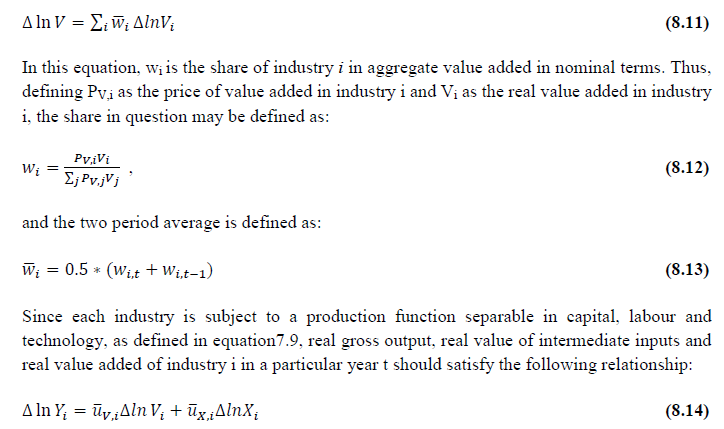 In this equation, uV and uX are the shares of value added and intermediate inputs in the gross value of output in nominal terms. Given data on growth in gross output and growth in intermediate input of a particular industry, the above equation yields the growth in real value added of that industry. TFP growth from the aggregate production possibility frontier may be defined as follows:  In this equation K and L are aggregate capital input and labour input respectively, and vK and vL are value shares (or income shares) of capital and labour respectively. If one maintains the assumption that each specific type of capital and labour input has the same price in all industries, then each type of capital (labour) can be summed across industries and then a Törnqvist index can be constructed to yield aggregate capital (labour) input. Alternatively, different types of capital input can be combined using a Törnqvist index into total capital input used in an industry and then industry level growth in capital input can be combined with the help of a Törnqvist index to obtain growth in capital input at the aggregate level. In a similar manner, the growth in aggregate labour input can be computed. The third approach to measuring the TFP index at a higher level of aggregation is to apply direct aggregation to industry level estimates. This maintains the industry level production accounts as the fundamental building block and begins with industry level sources of growth. Of the three approaches described here, this is the least restrictive in terms of the assumptions involved. The following equation expresses the relationship between aggregate value added growth and the growth in capital and labour inputs and TFP in individual industries:  In this equation, vK is the value share of capital in gross output, vL is the value share of labour in gross output, vV is the share of value added in gross output, and wi is the share of industry i in aggregate value added in nominal terms. The bars indicate that the average of two periods, t and t-1, are to be taken. The last term in equation 7.16 is:  This is the Domar aggregation of TFP growth rates at individual industry level. Note that it is weighted average of industry level TFP growth rates. But, the weights add up to more than one. The data constructed for gross value added and gross output, labour input, capital inputs, intermediate inputs and factor income shares (Chapters 2, 3, 4, 5, 6 and 7 respectively), are used to estimate TFPG during the period 1980 to 2015. Labour input is measured using total person worked (see, Chapter 4 for the detailed discussion). The series on growth rate in capital services is taken from Chapter 5. 1 Timmer, M.P, Mahony, M. and van Ark, B.(2007). The EU KLEMS growth and productivity accounts: an overview. Mimeo University of Groningen & University of Brinmingham, 2 Readers can refer to India KLEMS Data Manual Version 2013 for the data set released by RBI on its website in June 2014. 3 From both aggregated 9 NAS sectors Gross Domestic Product by economic activity statement along with the disaggregated statements of these 9 NAS sectors. 4 It uses NAS Series 2004-05 for more recent years. 5 Kanhaiya Singh and M.R. Saluja (2016), Input-Output Table for India, 2013-14, Working Paper no WP-111, National Council of Applied Economic Research, New Delhi 6 The principal components of Manufacturing n.e.c are Manufacturing of jewellery and related articles, Manufacture of musical instruments, Manufacture of sports goods, Manufacture of games and toys and other manufacturing. 7 See Himanshu (2011) for a discussion on many issues associated with the NSSO employment surveys. 8 The interpolation methodology and the use of other sources for few industries is explained in the subsequent section. 9 The coverage and the sample size of thin rounds is different from major rounds. 10 Problems in using UPSS are: The UPSS seeks to place as many persons as possible under the category of employed by assigning priority to work; no single long-term activity status for many as they move between statuses over a long period of one year, and Usual status requires a recall over a whole year of what the person did, which is not easy for those who take whatever work opportunities they can find over the year or have prolonged spells out of the labour force. 11 In EU-KLEMS changes in labour composition has been measured by including employment class, gender, age and education (Timmer,op cit; p64) and only 3 categories of education defined as high skilled, medium skilled and low skilled have been taken. This concept of labour composition is refereed as ‘labor quality’ by Jorgenson. It is recognized (Timmer; op cit; p84) that the categorization may lead to biases in the aggregate composition adjustment if employment trends and wage share differ within categories. These education categories generally correspond to- up to Primary education, above Primary to Hr Secondary education and above Hr Sec or College education. Due to data limitations in India we have measured changes in labour composition only by changes in education profile of labour; hence named it labour education index. Therefore it became necessary to have a more detailed classification of education to capture the changes in skill composition of labour in India. For comparison, we estimated the changes in labour composition based on three education categories also and found that for the total economy the annual trend growth in labour education index is 1.16 percent as compared to 1.25 percent based on five education categories. 12 This procedure has been advocated by NSSO itself and has been consistently adopted by almost all researchers. 13 A very lucid description of the same is given by Sivasubramonian (2004). 14 Appendix Table 1 provides the details about the Census Population, WFPR by UPSS, and persons employed in each of the EUS rounds used in the study. 15 The 66th round has not been used because of its inconsistency with the 61st and 68th round. Most economists consider it as an outlier. 16 Since 2009-10, the labour Bureau, GOI has started collecting annual data on Employment and Unemployment and has released five reports till 2015-16. Its estimates are not comparable with EUS and the unit level data, which is used to get employment by different characteristics-age, gender, education, etc. is also not provided. So only the growth rates provided by Labour Bureau data are used in the KLEMS employment series. 17 Aggregate input is measured as a translog index of its individual components. Then the corresponding index is a Törnqvist volume index (see Jorgenson, Gollop and Fraumeni 1987). For all aggregation of quantities we use the Törnqvist quantity index, which is a discrete time approximation to a Divisia index. This aggregation approach uses annual moving weights based on averages of adjacent points in time. The advantage of the Törnqvist index is that it belongs to the preferred class of superlative indices (Diewert 1976). Moreover, it exactly replicates a translog model which is highly flexible, that is, a model where the aggregate is a linear and quadratic function of the components and time. 18 Although census population is available only decennially, we used the interpolated population figures for the mid-year survey periods [Visaria, (1996) for 1977-78 (Jan) and 1987-88 (Jan); Sundaram, (2007) for 1983 (July), 1993-94 (Jan), 1999-00 (Jan) and 2004-05 (Jan)] and from NSSO (2010) for Jan 2010 and Jan 2012. 19 In EU KLEMS (Timmer, op cit; p 67) it is assumed that the earnings is equal to the earnings of ‘regular' employees. 20 The details of the function can be obtained from the Stata software and from Appendix. 21 Asset prices are used in the aggregation of capital stock. However, it is the price of the capital service that must be used in aggregating capital services (see Jorgenson and Griliches, 1967; Diewert, 1980) as it is the services delivered by capital goods that are used in the production process. Jorgenson and Griliches (1967) have shown that these two prices are related; the asset prices are the discounted value of all future capital services. They are not proportional though, as there are differences in replacement rates and capital gains among different capital assets.  23 This version of the database does not make a distinction between ICT and non-ICT assets, as the industry level data on ICT assets are weak. An attempt to estimate aggregate economy level ICT capital can be found in Erumban and Das (2015). 24 See O’ Mahony and Timmer (2009) for a description of EU KLEMS database 25 This data is not publicly available. However, CSO has been kind to compile this data for the India-KLEMS project. 26 In some years transport equipment was provided as part of the machinery and equipment, categorized as ‘tools, transport equipment and other fixed assets’. In such cases, we use transport/tools, transport and other fixed asset ratio in the nearest year to separate transport equipment. 27 This choice is driven by the fact that the first year of availability of ASI data is 1964-65. 28 National Accounts Statistics-Sources and Methods, Chapter 26, CSO (2007) 29 We do not intend to delve into the controversies over the use of internal vs. external rate of return in the context of productivity measurement. Rather, given that this is the first version of our data, we use the external rate and in a later stage, we will also use internal rates. See Erumban (2008a and b) for a discussion on these issues. 30 Reserve Bank of India, Handbook of Indian Statistics, Annual volumes. 31 The estimation is done at group level rather than individual industries on the consideration that the group level estimates will be more reliable. 32 Consider, the semi conductor (SC) industry, which is a key input to the computer hardware industry. Much of the output is invisible at the aggregate level because semi conductor products are intermediate inputs to other industries rather than deliverables to final demand- consumption and investment goods. Moreover, SC plays a role in the improvements in quality and performance of other products like-computers, communication equipments and scientific instruments. Failure to account for them leads us to miss the role of key industries that produce intermediate inputs and importance of intermediate inputs for the industries that use them. ( Jorgenson, Ho and Stiroh (2005), Productivity, volume 3). |
|||||||||||||||||||||||||||||||||||
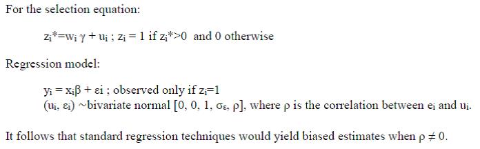
Measuring Productivity at the Industry Level - The India KLEMS Database
|
AUTHORS Deb Kusum Das Abdul Azeez Erumban Suresh Aggarwal Pilu Chandra Das Changes in India KLEMS Database 2018 over the India KLEMS 2017 version Overall
New Additions to KLEMS Variables
Certain Changes Made in Data Sources and Methodology Capital Input
Intermediate input
Factor Income Share
This document describes the procedures, methodologies and approaches used in constructing the India KLEMS database version 2018. This database is part of a research project, supported by the Reserve Bank of India (RBI) to analyse productivity performance in the Indian economy at disaggregate industry level. This work is meant to support empirical research in the area of economic growth. In addition, the database is meant to support the conduct of policies aimed at supporting acceleration of productivity growth in the Indian economy, requiring comprehensive measurement tools to monitor and evaluate progress. Finally, the construction of the database would also support the systematic production of reliable statistics on growth and productivity using the methodologies of national accounts and input-output analysis. In its definitive version the India KLEMS research project will include measures of economic growth, employment creation, capital formation and productivity at the industry level from 1980-81 onwards. The input measures will incorporate various categories of capital (K), labour (L), energy (E), material (M) and services (S) inputs. A major advantage of growth accounting is that it is embedded in a clear analytical framework rooted in production functions and the theory of economic growth. It provides a conceptual framework within which the interaction between variables can be analysed, which is of fundamental importance for policy evaluation. (Timmer et al., 2007)1. The present document describes the India KLEMS database version 2018. The present version is an extended India KLEMS research project, “Disaggregate Industry Level Productivity Analysis for India – the KLEMS Approach” being undertaken at the Centre for Development Economics, Delhi School of Economics. This one builds on the previous project, which was undertaken at ICRIER, New Delhi2. The Data Manual is intended to guide researchers about the variables (and their construction) used to measure both inputs and total factor productivity (TFP) at the industry level using the dataset. In addition, it is also intended to support national officials statistical agencies in future work on productivity database within the agencies. The dataset includes measures of Gross Value Added (GVA), Gross Value of Output (GVO), Labour (L) , Capital (K), Energy (E) , Material (M), Services (S), Labour Quality (LQ), Labour Productivity (LP) and Total Factor Productivity (TFP) at the industry and economy level from 1980-81 onwards. The database covering the period 1980-81 to 2016-17 has been constructed on the basis of data compiled from CSO, NSSO, ASI, Input-Output tables (I-O tables) and processed according to appropriate procedures. These procedures were developed to ensure harmonisation of the basic data, and to generate growth accounts in a consistent and uniform way. Harmonisation of the basic data has focused on a number of areas such as industrial classification, aggregation levels. The data base covers 27 industries comprising the entire Indian economy. The industries are shown in Table 1.1 below. The variables in the data set are given in Table 1.2. 1.2 Coverage: Industries and Variables In this section we describe the coverage of the India KLEMS database in terms of industries and variables. The time period covered is from 1980-81 (1980) to 2016-17 (2016). At a disaggregated level, database is created for 27 industries. The industrial classification is constructed by building concordance between NIC 2008, NIC 2004, NIC 1998, NIC 1987 and NIC 1970 so as to generate continuous time series from 1980 to 2016. This classification is very close to the International Standard Industrial Classification (ISIC) revision 3. The 27 industries are aggregated to form six broad sectors, namely:
Table 1.1 below provides a listing of the 27 industries, including the higher aggregates. Further the detailed classification and concordance of study industries with NICs is provided in Appendix. Table 1.2 provides an overview of all the series included in our database. Measures of capital (K), labour (L), energy (E), material (M) and service (S) inputs as well as gross output (GO), have been constructed using National Accounts Statistics (NAS), Annual Survey of Industries (ASI), NSSO rounds and Input-Output Tables (IO). In building annual time series on gross output, five inputs and factor income shares, various assumptions are made to fill up gaps in industry details and link series over time. As we know that NSSO rounds of unregistered manufacturing, Input Output Transaction Tables, and Employment and Unemployment Surveys by NSSO are available only for certain benchmark years. Thus, the use of information from these data sources necessitates interpolation and assumption of constant shares for building series of output and inputs. The construction of growth accounting series like total factor productivity, labour productivity are based on theoretical models of production and needs additional assumptions that are spelt out in subsequent chapters of the manual. Finally, the Other Series like NDP at factor cost, compensation of employees etc. are additional series which are used in generating the growth accounts and are informative by themselves. Chapter 2: Gross Value Added Series at the Industry Level For an individual firm or industry, productivity measure can be based on a value added concept where value added is considered as an industry’s output and only primary inputs such as labour and capital are considered as industry input. Value added based productivity measures reflect an industry’s capacity to contribute to economy wide income and final demand. In this sense they are valid complements to gross output based measures. This chapter describes the data sources and methodology used to construct the Gross Value Added (GVA) series at current and constant prices for 27 study industries for the period of 1980-81 (1980) to 2016-17 (2016). GVA of a sector is defined as the value of output less the value of its intermediary inputs. This value added created by a sector is shared among the primary factors of production, labour and capital. The National Accounts Statistics (NAS) brought out by the CSO (Central Statistics Office, Government of India) is the basic source of data for the construction of series on GVA for INDIA KLEMS-industries. NAS provides estimates of GVA (i.e., gross value added) for Indian economy at a disaggregate industry level at both current and constant prices for the period since 1950-51. CSO provide GVA at constant (2011-12) prices onwards 2011-12, and prior to that at constant (2004-05) prices. Up to 2011-12, estimates of GVA at both current and constant (2004-05) prices for all industries are directly obtained from Back Series 2011 and NAS 2014. From 2011-12 onwards, estimates of GVA at both current and constant (2011-12) prices for all industries are directly obtained from NAS 2018. GVA series at current and constant (2011-12) prices are extended backwards up to 1980-81 using annual growth rate estimated from Back Series 2011 and NAS 2014 (this has been done in order to construct India KLEMS GVA series with base 2011-12). NAS estimates of value added for a few industry groups are at a more aggregate level, requiring the splitting of the aggregates. In such cases, the NAS estimates of value added have been split to obtain estimates of value added at a higher level of disaggregation. NAS provide separate estimates of GVA for registered and unregistered manufacturing. However, onwards 2011-12 NAS disaggregated the manufacturing sector in corporate sector and household sector. For splitting the aggregate estimates of GVA for registered manufacturing industries and corporate sector, we have used data from the Annual Survey of Industries (ASI) based on the National Industrial Classification 2004 and 2008 (NIC-2004 & NIC-2008). Whereas, for the unregistered manufacturing sector, we have used results from six rounds of NSSO surveys- [40th (1984-85), 45th round (1989-90), 51st round (1994-95), 56th round (2000-01), 62nd round (2005-06), 67th round (2010-11) and 73rd round (2015-16)] to obtain value added estimates. In India, GDP for unregistered manufacturing is constructed using the labour input method. The estimates of GVA for the unregistered manufacturing sector are obtained as a product of the work force and the corresponding GVA per worker. The information about employment in the unorganised sector is only available in the benchmark years for which NSSO survey data are available. Therefore, there is no consistent source of employment data for the years between these Quinquennial surveys. Even the information on value added per worker is equally limited, since the value-added data are also updated on an approximate 5-year interval (for details, see CSO, 2007). Therefore, estimates of value added for the unregistered manufacturing sectors for the years between the benchmarks have been obtained by interpolation and for years outside the benchmark years by linear extrapolation. For splitting the aggregate estimates of GVA for household sector for recent years (i.e., 2011 onwards), we have used GVA data from 67th round (2010-11) and 73rd round (2015-16). The construction of Gross valued added series involves three steps. Step 1: A concordance table between the classification used in the NAS and the 27 study industry classification used for this project has been prepared. Further, concordance between all the 27 sectors has been constructed with NIC - 1970, 1987, 1998, 2004 and 2008. Out of the 27 study industries, for 20 industries, GVA series both in current and constant prices is directly available from NAS3. The sectors for which data are provided in NAS are Agriculture, Forestry & logging, Fishing, Mining and Quarrying, Manufacturing (registered and un-registered), Electricity, Construction, Trade, Hotels & Restaurants, Railways, Transport by other means, Storage, Communication, Banking & insurance, Real estate, Ownership of Dwelling & Business Services, Pubic Administration & Defense and Other Services. Step 2: For manufacturing industries where direct estimates of GVA were not available from NAS, estimates have been made using additional information from ASI and NSSO unorganised manufacturing data. For 6 out of 13 manufacturing sectors GVA data are directly available from NAS. The list of these industries is provided in the table below. For the remaining 7 industries GVA data is constructed by splitting the NAS data using ASI or NSSO distributions. ASI data (annual) has been used for registered manufacturing whereas interpolated ratios from NSSO 40th (1984-85), 45th (1989-90), 51st (1994-95), 56th (2000-01), 62nd (2005-06), 67th round (2010-11) and 73rd round (2015-16) rounds have been used for Unregistered Manufacturing segments. A list of study industries is presented in Table 2.2 showcasing the methodology used to split GVA of certain NAS sectors to match concordance with our classification. It is important to note that the industry level value added volume indices are based on NAS. CSO provides single deflated value added estimates for all sectors except Agriculture. Following are the details of steps taken in splitting NAS sectors into India KLEMS industries for which direct GVA series are not available. Wood and wood products and manufacturing of furniture NAS back-series 2011 (based on 2004-05 prices) provides GVA of Wood and Wood products, furniture, fixtures etc. (20+361) for registered and unregistered manufacturing sectors. Since 2004-05 (from NAS2011 onwards) we have separate series for Wood and Wood products (20) and Manufacturing of furniture and fixtures (361). For our study, we need these two industries separately and 20 would be India KLEMS sector 20 and 361 would be part of India KLEMS Manufacturing n.e.c and Recycling (36+37) i.e., 361 would be added to 369+37. Thus since 2004-05, we have used the separate GVA series of Wood and Wood Products (20) and Manufacturing of furniture (361) obtained directly from NAS disaggregated series of registered and unregistered statement of GDP by economic activity. NAS back-series 2011 of GVA of Wood and Wood products, furniture, fixtures etc. (20+361) for registered manufacturing from 1980-81 to 2003-04 has been split using the ratio of GVA at current price of Wood and Wood Product (20) to Manufacturing of furniture (361) obtained from Annual Survey of industries (ASI). In case of unorganised manufacturing GVA for these two industries, separate GVA series have been obtained by using the ratio created from NSS unorganised manufacturing surveys of the benchmark years. The ratio of GVA for the interim years between two benchmark years have been linearly interpolated till 2003-04, and from 1980-81 to 1984-85, the ratio of 1984-85 has been used.4 Coke, Refined Petroleum Products and Nuclear Fuel and Rubber and Plastic Products We split ‘rubber, petroleum products’ (which are clubbed under one group in NAS) to arrive at two industry groups i.e., Coke, Refined Petroleum Products and Nuclear Fuel (23) and Rubber and Plastic Products (25). For the organised segment, we use the ASI (annual) data to get the individual sector shares and split the NAS data using these individual shares. Likewise, we use the relevant data from the four NSS surveys mentioned earlier to get the individual sector shares for the unorganised segment of this sector. The ratio of GVA for the interim years between two benchmark years have been linearly interpolated till 2003-04, and from 1980-81 to 1984-85, the ratio of 1984-85 has been used. Basic Metals and Fabricated Metal Products In our industry classification, basic metals and fabricated metal products (27+28) and machinery (29) are separate groups whereas ‘manufacture of fabricated metal products’ (28); ‘manufacture of machinery and equipment n.e.c’ (29) and ‘manufacture of office, accounting and computing machinery’ (30) are clubbed together as metal products and machinery (28, 29 and 30) in NAS. To arrive at individual industry result, we use ASI shares for organised sectors and NSSO surveys for the unorganised sector. We add to the fraction of fabricated metal products (28) from metal products and machinery to basic metals (271+272+2731+2732) already available. Electrical and Optical Equipment In our study classification, ‘electrical and optical equipment’ includes all sectors from 30 to 33. However, ‘electrical machinery’ in NAS includes industries ‘manufacture of electrical machinery and apparatus n.e.c.’ (31) + ‘manufacture of radio, television and communication equipment and apparatus’ (32) and excludes ‘manufacture of office, accounting and computing machinery’ (30) and ‘manufacture of medical, precision and optical instruments’ (33). However, 30 is part of ‘metal products and machinery’ and 33 is part of ‘other manufacturing’ in NAS. We take out 28 from metal products and machinery in NAS, with 29 and 30 being left, which we split using ASI. NSSO surveys have been useful here as well to compute the unorganised segment share. Likewise, we also take out the share of 33 from ‘other manufacturing’ in NAS separately for both organised and unorganised segments to arrive at GVA for electrical and optical equipment. Step 3: According to India KLEMS, output is adjusted for Financial Intermediation Services Indirectly Measured (FISIM). The value of such services forms a part of the income originating in the banking and insurance sector and, as such, is deducted from the GVA. The NAS provides output net of FISIM for some industry groups at a more aggregate level. For instance, in the estimates of GVA obtained for the registered manufacturing sector, adjustment for FISIM in NAS is made only at the aggregate level in the absence of adequate details at a disaggregate level. However, we have allocated FISIM to all the sectors of manufacturing by redistributing total FISIM across sectors proportional to their sectoral GDP shares. Similar redistribution of FISIM has been done in case of Trade sector and Other Services sector. First, the value added series presented in the project are at factor cost (as published in NAS), however, according to the KLEMS methodology as adopted in EU KLEMS , value added data has to be presented in basic prices as adopted in System of National Accounts 1993 (SNA 1993). However, the basic price is the amount receivable by the producer from the purchaser for a unit of a good or service produced as output minus any tax payable, and plus any subsidy receivable, on that unit as a consequence of its production or sale. It excludes any transport charges invoiced separately by the producer. Secondly, in order to make international comparisons, we need to convert the given ‘GDP at factor cost’ to ‘GDP in basic prices’. For this, we require net indirect taxes on production (indirect taxes less subsidies) for 27 industries and for every year since 1980. At present, we have GDP at basic prices from 2004-05 to 2016-17 for some industries of India KLEMS, which has been provided to us by CSO according to the NAS industrial classification. Since the information about indirect taxes and subsidies is not readily available for 27 study industries and also for the given time period, the challenge is to extend the series backwards by splitting up aggregate indirect taxes and subsidies data. Chapter 3: Gross Output Series at the Industry Level This chapter describes the procedures and methodologies used in constructing the database for gross output series at the industry level over the period 1980-81(1980) to 2016-17(2015). We discuss both the raw data sources and the adjustments that have been made to generate the time series on output and value added consistent with the official National Accounts. The methodology for measuring industry output, and value added was developed by Jorgenson, Gallop and Fraumeni (1987) and extended by Jorgenson (1990 a). Following a similar approach as explained in Jorgenson et al., (2005, Chapter 4) and Timmer et al., (2010, Chapter 3), the time series on gross output and intermediate inputs for the Indian economy have been constructed. The gross output of an industry is defined as the value of industry production using primary factors like labour, capital and intermediate inputs purchased from other industries. The gross output production function is separable in inputs and technology. An important advantage of gross output approach is that it provides a complete measure of production and treats all inputs - labour, capital and intermediate inputs symmetrically. In contrast the value added measure of output does not explicitly account for the flow of intermediate inputs which may be the primary component of an industry’s output. We use the more restrictive value added concept primarily because it is useful for aggregation purposes. It is to be noted that aggregate output (aggregated over industry value added) is a value added concept and the detailed methodology of aggregation of output across industries is explained in chapter 8. To construct the gross output series at industry level we use multiple data sources namely National Accounts Statistics, Annual Survey of Industries, NSSO rounds for unorganised manufacturing and Input Output Transaction tables. The data source and methodology used are documented below: National Accounts Statistics: The National Accounts Statistics (NAS) published by the CSO (Central Statistics Office, Government of India) is the basic source of data for the construction of time series on gross output. NAS provides estimates of gross output (GVO) for Indian economy at a disaggregate industry level at current and constant prices since 1950-51. Gross output data is available in NAS for Agriculture, Mining and Quarrying, Construction and Manufacturing sectors (Registered and Unregistered Manufacturing). From 2011-12 onwards, estimates of GVO at both current and constant (2011-12) prices for all industries are directly obtained from NAS 2018. GVO series at current and constant (2011-12) prices are extended backward up to 1980-81 using annual growth rate estimated from Back Series 2011 and NAS 2014. (a) Filling procedures of National Accounts series: It is to be noted that the NAS estimates of gross output for a few industry groups are at a more aggregate level, requiring splitting of the aggregates. In such cases, NAS estimates of output have been split using additional information from Annual Survey of Industries and NSSO rounds of Unregistered Manufacturing to obtain estimates at higher level of disaggregation. Secondly, for Unregistered manufacturing gross output data is available in NAS from 2004-05 onwards. In this case, information from NSSO survey rounds has been used for missing years to derive output estimates of unregistered manufacturing industries at current and constant prices. Annual Survey of Industries and NSSO Quinquennial Survey Reports: As mentioned above, gross output data are available at a more disaggregated level in Annual Survey of Industries (ASI) and NSSO Quinquennial surveys for Registered and Unregistered Manufacturing industries, respectively. These secondary data sources are used in this study for two purposes: (a) in certain cases NAS provides combined estimates of GVO and GVA for two manufacturing industries. In such cases separate estimates for individual study industries are obtained with the help of ASI or NSSO unorganised manufacturing sector data. (b) For the period prior to 2004, NAS does not provide estimates of GVO for unorganised manufacturing industries. To make our estimate of GVO for this period, the NSSO data are used. The Major NSSO Rounds for Unregistered Manufacturing used are 40th Round (1984-85), 45th Round (1989-90), 51st Round (1994-95), 56th Round (2000-01), 62nd Round (2005-06), 67th round (2010-11) and 73rd round (2015-16). Input-Output Transaction Tables: As motioned earlier, for GVA series of service sectors we obtain our estimates from NAS. However, prior to 2011-12 National Accounts do not provide any estimates of gross output of service sectors and hence we rely on Input-Output transaction tables which are available at an interval of 5 years or so. This necessitates interpolation and assumption of constant shares for measuring output of services sectors. The Input-Output transaction tables for benchmark years of 1978-79, 1983-84, 1989-90, 1993-94, 1998-99, 2003-04, 2007-08 and 2013-14 (prepared by National Council of Applied Economic Research5 (NCAER)) are used to derive gross output series for service sectors. The construction of the gross output series from 1980 to 2016 at current and constant prices involves the following steps: Step 1: Measuring Gross Output of Agricultural Sector, Mining and Quarrying, and Construction NAS provides nominal and real GVO series for a) Crops and Plantation, b) Animal Husbandry c) Forestry and Logging d) Fishing. By aggregating the GVO of these four subsectors we derive the GVO of Agricultural sector. The Gross output estimates of Mining and Quarrying and Construction at current and constant prices from 1980-2016 is also directly taken from NAS. Step 2: Measuring Gross Output of Manufacturing Industries For manufacturing industries time series on gross output is obtained by adding the magnitudes for registered and unregistered segments of manufacturing. As mentioned earlier, NAS estimates of gross output for manufacturing industries are at a more aggregate level. In such cases the aggregate output of NAS at current prices has been split using additional information from ASI and NSSO unorganised sector reports. Gross output data for 6 out of 13 manufacturing industries listed in table 3.1 are directly picked up from NAS. For the remaining 7 industries, output is constructed by splitting the NAS output data using ASI or NSSO distributions. ASI data (annual) has been used for registered manufacturing whereas interpolated ratios from NSSO 56th (2000-01), 62nd (2005-06), 67th (2010-11) and 73rd (2015-16) rounds have been used for unregistered manufacturing segments. A list of study industries is presented in Table 3.2 showcasing the methodology used to split GVO of certain NAS sectors to match concordance with our classification. The detailed method of splitting the output of NAS sectors to derive output of individual industries is given as follows: Basic Metals and Fabricated Metal Products; Machinery, n.e.c.; Electrical and Optical Equipment Metal products and Machinery of NAS is split into three parts: Manufacture of Fabricated Metal Products, Manufacture of Machinery and Equipment, Manufacturing of Office Accounting and Computing Machinery. For registered segments individual industry shares from ASI are used to split the data. For unregistered segments sectoral shares are calculated from 56th (2000-01), 62nd (2005-06), 67th (2010-11) and 73rd (2015-16) NSSO rounds of unregistered manufacturing. The shares for interim years have been estimated by interpolation and applied to the combined output of NAS to split it into three industries. Machinery forms a separate study sector. Next, a fraction of Manufacture of Fabricated Metal Products is added to Basic Metals of NAS to form output for study sector Basic Metals and Fabricated Metal products. A fraction of Manufacturing of Office Accounting and Computing Machinery is added with Electrical Machinery and Manufacture of Medical and Optical Instruments to form Electrical and Optical Equipment sector. Coke, Refined Petroleum Products and Nuclear Fuel; Rubber and Plastic Products We split ‘rubber, petroleum products’ (which are clubbed under one group in NAS) to arrive at two industry groups, i.e., Coke, Refined Petroleum Products and Nuclear Fuel (23) and Rubber and Plastic Products (25). For the registered segment, we use the ASI (annual) data to get the individual sector shares and split the NAS data using these individual shares. Likewise, we use the relevant data from the four NSS surveys mentioned earlier to get the individual sector shares for the unregistered segment of this sector. Wood and Products of Wood; Manufacturing, n.e.c.; Recycling NAS back-series 2011 (based on 2004-05 prices) provides GVO of Wood and Wood products, Furniture, Fixtures etc. (20+361) for Registered and Unregistered Manufacturing segments. Since 2004-05 (from NAS2011 onwards) we have separate series for Wood and Wood products (20) and Manufacturing of furniture and fixtures (361). In our study, Wood and Wood Products (20) form a separate industry. Manufacturing of furniture and fixture (361) adds up with Manufacturing n.e.c6 (369) and Recycling (37) to form study industry Manufacturing n.e.c and Recycling. Thus since 2004-05, we have used the separate output series of Wood and Wood Products (20) and Manufacturing of furniture (361) obtained directly from NAS disaggregated series of registered and unregistered segments of GDP by economic activity. Prior to 2004, we use ASI data for registered segments to spit the NAS sectors to arrive at estimates of individual study industry. Prior to 2004, we observed some fluctuation in the estimated GVO series for Manufacturing, n.e.c.; Recycling industry. We tried to correct that by applying GVO to GVA ratio to GVA estimates. These ratios are separately obtained from ASI and NSSO survey rounds and then combined using organised and unorganised industry share in aggregate value added. However, for the period prior to 2004, separate output estimates for Unregistered Manufacturing segments are not available in NAS. Thus, to estimate output of Unregistered Manufacturing for the period 1980 to 2003 the following has been done.
Step 3: Measuring Gross Output for Services Sectors and Electricity, Gas and Water Supply Onwards 2011-12 NAS provided estimates of GVO at current and constant prices. Prior to 2011-12 Gross Output series for Services sectors and Electricity, Gas and Water Supply has been constructed using information from Input-Output Transaction Tables of the Indian economy published by CSO.
Firstly, the present study provides estimates for manufacturing and its sub-branches without segregating manufacturing (and its sub-branches) into organised and unorganised segments. However, given the employment potential and sizable presence of the unorganised segment in many of the manufacturing industries, it would be worthwhile in the Indian context to examine separately the productivity performances of both the organised and unorganised components. Some work to construct the output and input series separately for organised and unorganised components of Indian manufacturing has been done. A paper based on this analysis has been prepared. The data series for organised and unorganised manufacturing is not included in this release of India KLEMS database. Finally, National Accounts do not provide any estimates of gross output of services sector and hence we rely on IOTT which are available at an interval of about 5 years. This necessitates interpolation and assumption of constant shares for measuring output of services sectors. This issue is analogous to those explained in Timmer et al., (2010, Chapter 3) for the EU economy. Griliches (1994) paid particular attention to services sector output as a key source of uncertainty. Chapter 4: Labour Input Series at the Industry Level This chapter provides information on the sources of data and method of measuring labour services. The aim is to estimate labour input so that it reflects the actual changes in the quantity (number of persons) and quality of labour input over time. Labour input is measured by combining data on labour persons and data on labour quality. In the KLEMS framework it is desirable to estimate changes in labour composition by industries on the basis of age, gender and education. The measurement of labour composition is essentially an attempt to distinguish one labour type from the other taking into account the embodied human capital in each person. The source of human capital could be through investment in education, experience, training, etc. The contribution to output by each person also comes from this embodied capital and the reward (wages and earnings) to each person also includes the reward for investment in human capital. Therefore, it is essential to separate out these differences in labour to clearly understand the underlying differences in labour characteristics. It is in this context that an initiative has been taken to estimate labour composition index. Nevertheless, many limitations of India’s employment statistics, especially the availability of information on wages/ earnings of different category of workers which could be used as an indication of their differences in ability makes it difficult to quantify these changes in the labour force in a pertinent way. The problems of employment statistics in India has been widely discussed in the literature (Sivasubramonian; 2004, & Himanshu; 2011). The KLEMS project aims to build a time series of employment series for 27 industrial sectors. However, there exists no time-series data on employment for the Indian economy, except for the organised segment. Therefore, it was essential to make certain assumptions regarding the annual changes in the employment series using available information. Subsequently we discuss these issues in detail. The large scale Employment and Unemployment Surveys (EUS) by National Sample Survey Organization (NSSO)7 and the estimated population series based on the decennial population census are the main data sources for estimating the workforce by industry groups, as per the National Industrial Classification (NIC). The other data sources on employment are Economic Survey (for public enterprises), Annual Survey of Industries (ASI for organised manufacturing Industries) and Labour Bureau Surveys (available since 2009-10). Interpolated population is used for intervening years8. In India, major or Quinquennial rounds of EUS which have been conducted by NSSO since 1980 are 38th (1983), 43rd (1987-88), 50th (1993-94), 55th (1999-2000), 61st (2007-08), 66th (2009-10) and 68th (2011-12) rounds. The major round 32nd (1977-78) has been used for extrapolating the labour series to 1980-81. Since 1989-90, the NSSO has also conducted annual surveys with small sample sizes. While the annual surveys or thin rounds have shorter reference periods, six months in some cases, they also have limited coverage. The thin rounds relate to both rural and urban sectors of the economy. So while some economists have preferred to ignore them almost completely (Sundaram, 2007), others have supported their use (Bhalla and Das, 2005; Srinivasan, 2008). Because of the limitations of thin rounds9, they have not been used in constructing the time series of labour input. In the NSS surveys, the workers are classified on the basis of their activity status into usual principal status (UPS), usual principal and subsidiary status (UPSS), current weekly status (CWS) and current daily status (CDS) for Quinquennial rounds (also known as major rounds) and Usual Status & CWS for annual rounds (also known as thin rounds). While UPS, UPSS and CWS measure number of persons, the CDS gives number of person days. UPSS is the most liberal and widely used of these concepts and despite its limitations10 this seems to be the best measure to use given the data. UPSS, which includes all workers who have worked for a longer time of the preceding 365 days in either the principal or in one or more subsidiary economic activity has been used because of its advantages over others. Advantages of using UPSS, which gives number of persons employed, are: i) It provides more consistent and long term trend, ii) More comparable over the different EUS rounds, iii) NAS’s labour Input Method (LIM) is also now based on Principal and Subsidiary Status, and iv) Wider agreement on its use for measuring employment (Visaria, 1996; Bosworth, Collins and Virmani (BCV), 2007; Sundaram, 2008; Rangarajan, 2009). NSSO has used NIC 1970 for classification of workers by industry in 38th and 43rd rounds, NIC 1987 for 50th round, NIC 1998 for 55th and 61st rounds, NIC 2004 for 66th round and NIC 2008 for 68th round. Therefore as a starting point concordance between India KLEMS 27-sector industrial classification, and NIC-1970, 1987, 1998, 2004 and 2008 was worked out. There are, however, some data problems which need a mention:
Measuring Labour Persons at the Industry Level The construction of time series of labour input requires estimation of numbers of persons. While in India, number of persons has been used as a measure of labour input, OECD (2001) and EU KLEMS have estimated labour productivity in terms of output per labour hour worked. OECD does not favour using count of jobs and has published international comparisons of productivity for OECD countries that uses unadjusted hours. Efforts are made to estimate persons and adjust it for changes in labour composition by calculating the grand labour composition index, thus obtaining the composition change corrected labour input. The methodological issue is how to estimate number of persons employed. In India the total workforce in the country and its distribution over economic activities may be obtained from the decennial Population Census and the Employment and Unemployment Surveys (EUS) of the NSSO12. Out of the two, the latter are more dependable and have been used to assess the changes in employment and unemployment for employment planning and policy analysis. The preference for the use of EUS is generally based on the notion that prior to 2001, the three Censuses have clearly under reported the participation of women in economic activities; whereas the EUS has provided reasonably reliable estimates of the level and pattern of employment (Visaria, 1996). While Population Census underestimates work force participation rates (WPRs), the EUS estimates of total population are significantly lower than the Population Census based estimates – by over 20 percent in Urban India13. However, for the Census 2001, the WFPRs are closer to the rates from the 1999-2000 NSSO round. Due to these advantages of EUS, the present study has used the EUS14 for the survey years, i.e., till 2011-12. Thus, the surveys used are 38th, 43rd, 50th 55th, 61st and 68th rounds15. Between the survey periods interpolation of estimates was done to find employment for the intervening period. However, in few survey periods where the disaggregate employment of an industry was an outlier, it was ignored for interpolation and the interpolation in such cases was done between the other two adjacent rounds. The interpolation was supplemented by data from Economic Survey and ASI also. The growth rates, since 1984-85, from Economic Survey data has been used for the two industries- Electricity, Gas &water Supply; and Public Administration and Defence - where public sector mainly dominates. Similarly the growth in employment, since 1984-85, in the two other industries-Coke, Refined Petroleum products; and Transport Equipment, where a large proportion of employment is in the organised sector is taken from ASI. The interpolation of the employment series from 2012-13 to 2015-16 is based on the growth rates provided by the Labour Force surveys16 for the non-manufacturing industries. For the manufacturing industries, the growth rates obtained from the NSSO surveys of 67th round (2012-13) and 73rd round (2015-16) have been used for the unorganised manufacturing industries and the growth rates from ASI for the corresponding years have been used for the organised manufacturing industries. The estimates for the year 2016-17 are just extrapolated from the 2015-16 by using the average growth rates of employment between 2013-14 & 2014-15 and 2014-15 & 2015-16. The current employment series makes use of all the different available sources of data on employment to obtain a smooth and long time series which captures the relevant information provided by these sources. Between 2005 and 2015, we observed very high growth rate in number of employed persons series for the industry Electrical and Optical Equipment as compared to other manufacturing industries and the overall growth in employment in this industry during 2005-2015 was found to be higher than that for Construction (which seems somewhat unrealistic). It was also observed that there was a negative growth in employment in Textiles, Textile Products, Leather and Footwear although real GVA of this industry more than doubled between 2005 and 2015. To address these issues, some adjustments to the initial employment estimates for Electrical & Optical Equipment and Textiles, Textile Products, Leather and Footwear have been done. Onwards 2005, employment series for Electrical & Optical Equipment has been estimated applying annual growth rates obtained from ASI and NSSO rounds to the number of employed persons for the year 2005-06. Then, for the years 2005-06 to 2015-16, we compute the difference between estimated employment series from EUS rounds and that based on ASI & NSSO rounds for the Electrical and Optical Equipment industry and add it to Textiles, Textile Products, Leather and Footwear industry. This ensures that for the manufacturing as a whole our estimates remain the same as obtained from EUS rounds. Measuring Labour Composition Index The composition of labour force is of considerable importance in the context of productivity measurement, as it provides not only a more accurate indication of the contribution of labour to production but also the impact of compositional changes on productivity. Any improvement in labour skills or if proportions of each labour type in the labour force change, will have an impact on the growth of labour input beyond any change in total persons worked. It would increase the amount of labour input actually used in the process of production. One widely used methodology to capture changes in labour composition is given by Jorgenson, Gollop and Fraumeni (1987), which is that the aggregate labour input of sector ‘j’ is defined as a Törnqvist volume index of persons worked by individual labour types ‘l’ as follows:17 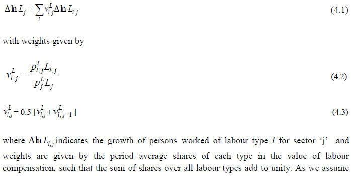  There is a second approach to the measurement of skill levels. The procedure is to use a simple index of educational attainment to adjust for skill differences. So improvement in educational attainment is adjusted by incorporating average years of schooling as the proxy for skill levels. For example, an index of the form: L* = easL assumes that each year of schoolings, raises the average worker’s productivity by a constant percentage, ‘a’. Such studies have been carried out for different time periods and for a large number of countries around the world, typically finding a return to each additional year of education in the range of 7 to 12 percent (BCV, 2007). Most of the recent indices of composition of labour input are based on the methodology of Jorgenson, Gollop, and Fraumeni (JGF) (1987) and uses the Törnqvist translog index. However, this methodology requires large volume of data. Using this methodology Aggarwal (2004) estimated labour composition for the Indian manufacturing labour force. There are however, lot of disagreements on the use of this methodology in the Indian context, as it assumes the existence of perfectly competitive labour markets where wage rate is the indicator of a person’s marginal productivity. The analysts argue that the observed wage differences may reflect factors other than productivity differences, such as age or gender. Its use is also questioned because data for large segment of Indian labour force- the self -employed is not available. Since the Indian labour market is still not very competitive and there are data weaknesses, therefore the researchers in India have generally avoided applying the JGF methodology. For this reason, most Indian researchers have avoided to account for the differences in age and gender characteristics. However, to account for educational differences they have preferred to exercise either of the two choices- one to use Barrow and Lee (1993) methodology and presume a constant rate of return for education (BCV, 2007) or second is to use the limited information available on wages for few rounds and only for casual and regular employees (Sivasubramonian, 2004) to determine the weights of different types of persons. Bosworth and Collins (2008) assumed a constant annual return of 7 percent for each additional year of education irrespective of the level of education. The problem with the assumption of uniform returns for each year is that it ignores all variations- across levels of education, over gender, over age groups, over industries, etc. and only includes education. It is thus not able to capture the impact of change in gender composition, age composition (a proxy for experience) and industry composition. The present version of the manual has included only one of these characteristics and a Grand labour composition index has been estimated based on JGF methodology using suitable data. The gender characteristic is avoided as Indian females still have very low level of education in general and higher education in particular, especially among the middle and senior age group. Therefore, either no data is available or there are very few sample observations for many such cells with cross classification of education, age and industry. The data for the survey years on total number of persons employed by each industry is taken from the current employment series. The estimates for the year 2016-17 are just extrapolated from the 2015-16 by using the average growth rates of labour quality between the last two rounds. The data on employment is essentially derived from the unit level record data of National Sample Survey (NSS) which is made available by NSSO in the form of CD-ROMS for the five Quinquennial rounds beginning from 38th. We estimated the number of employed persons according to UPSS as follows:
For extrapolation backward to 1980-81 to 1982-83, the interpolation of the broad industrial classification of 32nd round and 38th round is used. So the estimates from 32nd round are mainly used as control numbers. For the construction of the labour composition indices we require data on employment and earnings by education for the broad sectors and for each of the 27 industries. We distinguish three types of educational categories for broad sectors and three types of educational categories for each of 27 industries because of large data requirement at disaggregate level. The three education categories used are ‘up to primary’, ‘above primary to higher secondary’, and ‘above higher secondary’. Therefore the following additional steps have also been performed:
Secondly, earnings of self-employed have also been estimated from the monthly consumption expenditure of these households. In this, first the total monthly consumption expenditure is divided by the number of employed persons in the household to get total monthly consumption expenditure per employed person. Then the ratio of wage earnings by total monthly consumption expenditure per employed person has been calculated for each industry by UPSS status for the selected rounds. Assuming the consumption earnings ratio to be same for casual and self-employed persons, the ratio for casual labour is used for self-employed persons and this ratio is multiplied to the total monthly consumption expenditure per self-employed person so as to get the earnings of the self-employed persons. However, if the earnings thus obtained are higher than the earnings obtained from Mincer equation, then the latter are used. So the lower of the two - earnings obtained from Mincer equation or the earnings based on consumption expenditure, are taken to be the earnings of the self-employed persons. Once the above steps are taken to find out the educational distribution of all employed persons in all the five rounds and their corresponding wages, the computation of the grand labour composition index is carried based on the JGF (1987) methodology with 1980-81 equal to 100. The index is estimated for total persons working in 27 different industries in India for the 38th, 50th, 55th, 61st, and 68throunds of NSSO with 1983 (38th round) equal to 100 so as to assess the temporal changes in labour skill. Since the series required is from 1980-81, we have extrapolated it backwards from 1983 to 1980-81. The next phase of this project aims to update the series and perform some robustness checks of the current employment series with the help of the next round of EUS data, which is expected in 2019 and bring out policy implications from the employment trends. Appendix C: Definitions of Employment in NSSO Employment & Unemployment Surveys The surveys of NSSO on employment and unemployment (EUS) aim to measure the extent of ‘employment’ and ‘unemployment’ in quantitative terms disaggregated by various household and population characteristics following the three reference periods of (i) one year, (ii) one week, and (iii) each day of the week. Based on these three reference periods three different measures, termed as usual status, current weekly status, and the current daily status, are arrived at. While all these three approaches are used for collection of data on employment and unemployment in the Quinquennial surveys, the first two approaches only are used for the purpose in the annual surveys. Usual principal status: In the NSS 27th round, the usual principal activity category of the persons was determined by considering the normal working pattern, i.e.,, the activity pursued by them over a long period in the past and which was likely to continue in the future. For the identification of the usual principal status of an individual based on the major time criterion, in NSS 27th, 32nd, 38th, 43rd rounds, a trichotomous classification of the population was followed, that is, a person was classified into one of the three broad groups ‘employed’, ‘unemployed’ and ‘out of labour force’ based on the major time criterion. From NSS 50th round onwards, the procedure was changed and the prescribed procedure was a two-stage dichotomous one which involved a classification into ‘labour force’ and ‘out of labour force’ in the first stage, and thereafter, the labour force into ‘employed’ and ‘unemployed’ in the second stage. Usual subsidiary status: In the usual status approach, besides principal status, information in respect of subsidiary economic status of an individual was collected in all employment and unemployment surveys. For deciding the subsidiary economic status of an individual, no minimum number of days of work during the last 365 days was mentioned prior to NSS 61st round. In NSS 61st round, a minimum of 30 days of work, among other things, during the last 365 days, was considered necessary for classification as usual subsidiary economic activity of an individual. Current weekly status: It is important to note at the beginning that in the EUS of NSSO, a person is considered as worker if he/she has performed any economic activity at least for one hour on any day of the reference week and uses the priority criteria in assigning work activity status. This definition is consistent with the ILO convention and used by most of the countries in the world for their labour force surveys. In NSSO, prior to NSS 50th round and in all the annual surveys till NSS 59th round, data on employment and unemployment in the CWS approach was collected by putting a single-shot question ‘whether worked for at least one hour on any day during the last 7 days preceding the date of survey’. The information so collected was used to determine the CWS of the individuals. This procedure was criticized for being not able to identify the entire workforce, particularly among the females. It was then decided to derive the CWS of a person from the time disposition of the household members for the 7 days preceding the date of survey. The procedure was used for the first time in NSS 50th round. It is seen that the change in the method of determining the current weekly activity had resulted in increasing the WPR in current weekly status approach - more so for the females in both rural and urban areas than for males. The trend observed in NSS 50th round in respect of the WPR according to CWS suggested continuing with the procedure for data collection in CWS in NSS 55th and NSS 61st rounds. Current Daily Status Current Daily Status (CDS) rates are used for studying intensity of work. These are computed on the basis of the information on employment and unemployment recorded for the 14 half days of the reference week. The employment status during the seven days is recorded in terms of half or full intensities. An hour or more but less than four hours is taken as half intensity and four hours or more is taken as full intensity. An advantage of this approach is that it is based on more complete information; it embodies the time utilisation, and does not accord priority to labour force over outside the labour force or work over unemployment, except in marginal cases. A disadvantage is that it relates to person-days, not persons. Hence, it has to be used with some caution.
Chapter 5: Capital Input Series at the Industry Level This chapter outlines the methodology employed to estimate capital services for the 27 industries in the India KLEMS database version 2018. Following an overview of the theoretical method developed by Jorgenson and Griliches (1967), and outlined in Jorgenson, Gollop and Fraumeni, (JGF, 1987), the Chapter discusses the specific empirical approaches we follow to implement these methods within the constraints of data availability for Indian industries. For the measurement of capital services we need capital stock estimates for detailed asset types and the shares of each of these assets in total capital remuneration. Using the Törnqvist approximation to the continuous Divisia index under the assumption of instantaneous adjustability of capital, aggregate capital services growth rate is derived as a weighted growth rate of individual capital assets, the weights being the compensation shares of each asset, i.e., 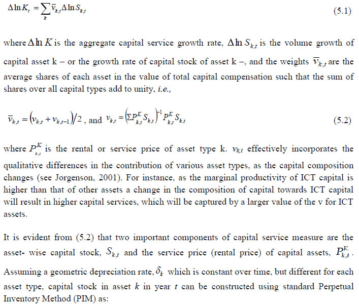 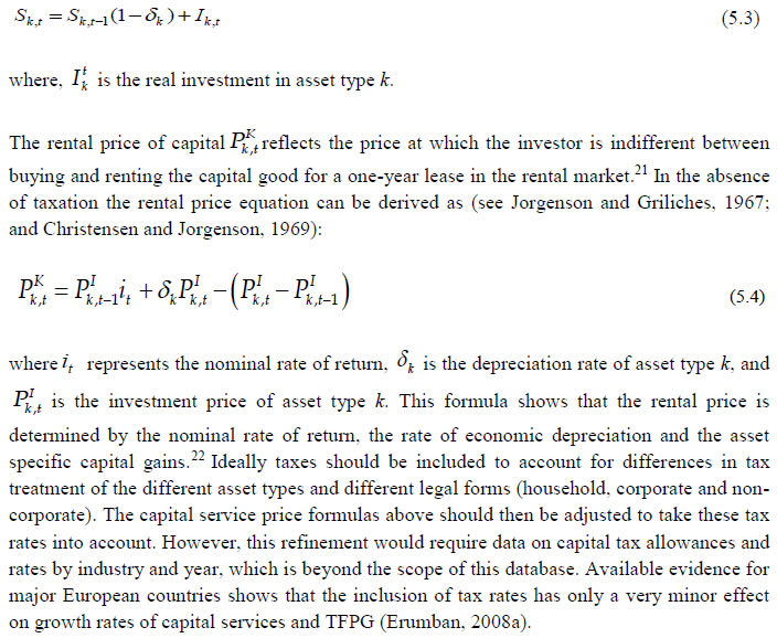 Since our measure of capital input takes account of asset heterogeneity, it was essential to obtain investment data by asset type. We distinguish between 3 different asset types – construction, transport equipment, machinery (includes ICT and non-ICT machinery).23 We exploit multiple sources of information for the construction of our database on capital services. This includes the National Accounts Statistics (NAS) that provide information on broad sectors of the economy, the Annual Survey of Industries (ASI) covering the organised manufacturing sector, the National Sample Survey Organizations (NSSO) rounds for unorganised manufacturing and Input-Output transaction tables. Even though we use multiple sources of data, our final estimates are fully consistent with the aggregate data obtained from the NAS. In addition, our approach to capital measurement is consistent with international practices such as the EU KLEMS24, which ensures the possibility of international comparisons. In what follows we discuss the various sources of data for asset-wise investment and the construction of the relevant variables, in detail. (a) Asset-wise investment for broad sectors of the economy Industry-level estimates of capital input require detailed asset-by-industry investment matrices. NAS provides information on aggregate capital formation by industry of use for 9 broad sectors, which, nevertheless, was not sufficient for our purpose. Therefore, we have collected more detailed data on assets and industries from the CSO.25 This is the data underlying the published aggregate gross fixed capital formation by the broad industry groups, separately for public and private sectors. For those sectors for which the investment matrices were not available from CSO, we gathered information from other sources (e.g. ASI for organised manufacturing and NSSO surveys for unorganised manufacturing) and benchmark it to the aggregate investment series from the National Accounts. The data used in the current version of the India KLEMS is based on the revised NAS with 2011-2012 base, and is available only since 2012. Therefore, for earlier years, we extrapolate the series using growth rates from previous version of the data. However, there were slight differences between the industry groups available in the current release of the data and the previous ones (see Table 5.1), which required some matching of sectors before combining the two series. Table 5.2 provides an overview of asset types available in NAS and their corresponding asset types used in our study. Investment in education and health are obtained directly from national accounts for the period after 2012, for each asset. For years before 2012, we assume the trend in the distribution of output, in order to split the total investment in the aggregates of these sectors into sub-sectors.
Total investment in each asset category is calculated as the sum of private and public sector investment in each asset. Investment in transport equipment is not available separately for private sector. We tried several approaches to impute the private sector transport equipment data. The first was to use the share of transport equipment in non-departmental enterprises. More specifically, we apply the non-departmental enterprise transport equipment to machinery & equipment (including transport equipment) ratio to machinery & equipment in private sector for each industry to obtain industry-wise transport equipment for private sector. We take non-departmental enterprises only, rather than the entire public sector, as it may be more realistic as it consists of public sector companies and statutory corporations, excluding administrative sector. However, the sum of industry estimates generated by this approach was not consistent with the reported aggregate private sector transport equipment. Therefore, we take a second step here, which is to use the industry distribution from this series and apply it to the published total private sector transport equipment data. The estimated transport equipment is then subtracted from each industry’s total machinery & transport equipment data, to obtain machinery in private sector as a residual. However, this approach generates many negative numbers in transport equipment in private sector, particularly in transport services. Therefore, we follow a third approach, which is what we finally use in the database. We first distribute the NAS total machinery in the private sector using the industry distribution of machinery and transport equipment. These estimates are then subtracted from each industry’s total machinery & transport equipment data to obtain the transport equipment investment in the private sector industries. (b) Asset-wise investment for non-NAS sectors NAS provides data only for 9 broad sectors, while we have 27 industries, which necessitated further splitting of some of the NAS sectors. This includes aggregate manufacturing (registered and unregistered separately) with 13 sub-sectors; other services into 4 sub-sectors; and real estate activities and business services into 2 sub-sectors. The manufacturing sector investment data was disaggregated into 13 sub-sectors at the 2-digit level of NIC 1998 using ASI and NSSO data, which will be discussed in detail subsequently. Investment series in service sector has been split into sub-sectors using two alternative approaches–value added shares, and capital/labour ratio in the higher aggregate industry. However, the final data used are based on value added shares, as a sensitivity analysis did not show a significant difference between the two. In order to split the aggregate capital formation in organised manufacturing sector into 13 study sectors, we use the Annual Survey of Industries. However, the published data does not provide any asset--wise investment information; it consists of only the aggregate capital formation or the book value of fixed capital. Most studies in the past have measured gross investment as the difference between book value of asset in period t and in period t-1 and add depreciation in period t to that. This approach has the deficiency of comparing two different samples reported in two different years, where the number of firms/factories might be different. In particular, while using this approach at industry level, for detailed asset categories, it might generate massive negative investment. We follow an alternative approach, following ASI’s definition of gross fixed capital formation (GFCF). ASI defines GFCF as actual additions (newly purchased, second hand and own construction) minus deductions plus depreciation adjustment for discarded assets during the year. This approach is based on a single year’s sample and helps to avoid potential huge negative investment series, and is also consistent with the published ASI GFCF series. The yearly detailed volumes beginning 1964-65 were used to derive the gross fixed capital formation by asset type directly. For the years 1964-1978, the relevant data are obtained from published detailed volumes. For the period, 1983-84 to 2004-05 ASI has generated detailed tables from Block C of ASI schedule that contain data on fixed assets. Data for missing years are interpolated using the changes in investment using book value method. Table 5.3 provides an overview of the asset categories available in ASI, and the relevant asset categories in our study to which they are attributed. Though ASI provides investment in land, for reasons of NAS consistency we exclude it from our database. Once investment in each of these assets and industries are generated using ASI data, we apply this industry-asset distribution to the published aggregate NAS GFCF series for organised manufacturing sector. It may also be noted that from 1960-61 to 1971-72, ASI data are for the census sector and from 1973-74 onwards they are for the factory sector. In order to make these two series comparable over years, we convert the data prior to 1972 to factory sector using the factory/census ratio in 1973. Thus, after these adjustments, we obtain investment data for 13 manufacturing sectors, by asset types, consistent with the NAS aggregates. The data required for creating the gross investment series for the 13 sectors of the unorganised manufacturing sector are obtained from various rounds of NSSO surveys on unorganised manufacturing. We use 6 rounds of NSSO surveys that cover the period 1989-2016. These are 45th round (1989-90), 51st round (1994-94), 56th round (2000-01), 62nd round (2005-06), 67th round (2010-11) and 73rd round (2015-16). Unit level data has been aggregated to 13 industries using the appropriate concordance tables. NSSO provides net addition to owned assets during the reference year within the block of fixed assets, and we use this as a measure of our investment. Asset classification in NSSO has changed over various rounds, and therefore, we have tried to match these with our classification as shown in Table 5.4. The investment series arrived at for four rounds were interpolated to obtain the annual time series of unorganised gross fixed capital formation by asset type. As in the case of registered sector, once the investment by asset types across industries are constructed, the asset-industry distribution is applied to the published NAS aggregate GFCF in unregistered manufacturing to obtain NAS consistent GFCF by asset type and industries. (c) Investment Prices by Asset Types In order to compute asset-wise capital stock using PIM (equation 5.3) and rental price (equation 5.4), we require asset-wise investment price deflators. Since CSO has provided us with investment data by industries and assets both in current and constant prices, we could derive the price deflators with base 2011-2012. For years before 2011, prices were spliced using 2004-2005 base investment deflators. These deflators are directly used for all the three asset categories we have. (d) Initial Stock, Depreciation Rates and Rate of Return As is evident from equations 5.1 to 5.4, our estimates of capital input require time-series data on asset-wise capital stock. Capital stock has been constructed using perpetual inventory method (PIM), where the capital stock (S) is defined as a weighted sum of past investments with weights given by the relative efficiencies of capital goods at different ages, which requires data on current investment by asset types, investment prices by asset types and depreciation rate. Also, for the practical implementation of PIM to estimate asset-wise capital stock, we require an estimate of initial benchmark stock (see Erumban, 2008b for an in-depth discussion on this issue). NAS provides estimates of net capital stock since 1950 for all the broad sectors in its Statement 17: Net Fixed Capital Stock by industry of use. We take the NAS estimate of real net capital stock in 1950 (in 1999-2000 prices) as our benchmark stock for all non-manufacturing sectors, and for manufacturing sectors the same is taken for the year 1964.27 However, since the NAS estimate is available only for broad sectors and for aggregate capital, we use our industry-asset distribution of GFCF in order to create net fixed capital stock estimates by asset type for all the 27 industries. NAS also provides detailed tables on assumed life of assets used for computing capital stock, for private units, administrative units as well as departmental and non-departmental units by asset types.28 We use these estimates of lifetime to derive appropriate depreciation rates for non-ICT assets, using a double declining balance rate. We assume 80 years of lifetime for buildings, 20 years for transport equipment, and 25 years for machinery and equipment. The final depreciation rates used in the study are given in Table 5.5 by asset type. Subsequently, we build our capital stock series by asset types for all the 27 industries using our GFCF series from 1950 (1964) onwards for the non-manufacturing (manufacturing) sectors. Our measure of capital input is arrived using equation (5.1), for which we also require estimates of rental prices (see equation 5.4). Assuming that the flow of capital services is proportional to the capital stock at individual asset level, aggregate capital flows can be obtained using a translog quantity index by weighting growth in the stock of each asset by the average shares of each asset in the value of capital compensation, as in (5.1). The rate of return (i) in equation (5.4) represents the opportunity cost of capital, and can be measured either as internal (or ex-post) rate of return, or as an external (ex ante) rate of return.29 This issue will be addressed in the further revisions of the data. The present version of the database uses an external rate of return, proxied by average of return on government securities and prime lending rate obtained from the Reserve Bank of India30. Therefore, we use a real rate, which is net of capital gain. Hence, the capital gain component in equation (5.4) is excluded while estimating rental price using external rate of return, obtaining  Where i* is the real rate of return, nominal interest rate adjusted for CPI inflation rate. Chapter 6: Intermediate Input Series at the Industry Level In this section we describe the basic approach we have used to derive the volume series of Intermediate Inputs namely – Energy input (E), Material input (M) and Services input (S). This breakdown of intermediate inputs can be used for extending the growth accounting exercises, but also convey interesting information about changing pattern in intermediate consumption ( see e.g. JHS 2005, chapter 4) The methodology for measuring industry output, intermediate inputs and value added was developed by Jorgenson, Gallop and Fraumeni (1987) and extended by Jorgenson (1990 a). The cornerstone of this approach is a time series of input-output (IO) tables which gives the flows of all commodities in the economy, as well as payments to primary factors. Every commodity is accounted for, whether produced by a domestic source or imported, and every use is noted, whether purchased by an industry or by a final demand element. All payments to factors of production i.e., labour and capital is accounted for so that all income elements of GDP are included. The methodology of constructing time series on energy, material and services inputs for the European economy has been elucidated in Timmer et al.,, (2010, Chapter 3). Following a similar approach as explained in Jorgenson et al., (2005, Chapter 4) and Timmer et al., (2010, chapter 3), the time series on intermediate inputs for the India KLEMS project have been constructed. Definition of EMS: As in EU KLEMS, this study identifies three main categories of intermediate inputs. They are classified as follows:
Intermediate inputs are broken down into energy, material and services, based on input-output transaction tables using a standard NIC product classification. The following five energy types (and products) have been classified as the Energy input.
The following fourteen input items have been classified as the Service input
All other intermediate inputs barring the above- mentioned nineteen inputs are classified as material input. The key building block for constructing time series on intermediate inputs at current prices, as explained in Jorgenson et al., (2005, Chapter 4), is the input-output transaction tables, that is, the inter-industry transaction tables that provide a description of which industries produce each product and which industries use them. The IOTT gives the inter-industry transactions in value terms at factor cost presented in the form of commodity x industry matrix where the columns represent the industries and the rows as group of commodities, which are the principal products of the corresponding industries. Each row of the matrix shows in the relevant columns, the deliveries of the total output of the commodities to the different industries for intermediate consumption and final use. The entries read down industry columns give the commodity inputs of raw-materials and services, which are used to produce outputs of particular industries. The column entries at the bottom of the table give net indirect taxes (NIT) (indirect taxes – subsidies) on the inputs and the primary inputs (income from use of labour and capital), i.e., Gross Value Added (GVA). As the IOTT is in the form of commodity x industry matrix, the row totals do not tally with the column totals. The difference between each column and the corresponding row totals is due to the inclusion of the secondary products, which appear particularly in the case of manufacturing industries. This is so because by-products are also manufactured by industries in addition to their main products. Thus, while determining the entries in the rows, a by-product of an industry is transferred to the sector (commodity row), whose principal product is the same as the by-product under reference. The columns, however, show the total of principal products and by-products of each industry. All the entries in the IOTT are at factor cost, i.e., excluding trade and transport charges and NIT. The Input Flow Matrix at factor cost, published by CSO, for 1978 is a 60 x 60 matrix. The absorption matrices for 1983, 1989, 1993 and 1998 have 115 sectors. However a detailed 130 sector absorption (commodity x industry) matrix for the Indian economy has been published from 2003-04 onwards. The scheme of sector classification adopted in supply use table 2012-13, IOTT 2007-08 and IOTT 2003-04 vis-à-vis, IOTT 1983-84, IOTT 1989-90, IOTT 1993-94 and 1998-99 has undergone significant change with the disaggregation of some of the sectors, which have become significant in early 2000s.
The methodology for computation of intermediate input series for 27 Industries from 1980-2016 at current and constant prices is explained in steps. Step 1: Concordance is done between IOTT and study industries
Step 2: Obtaining estimates for Material, Energy and Service Inputs for 27 Industries, in benchmark years
Thus, for each benchmark year, estimates are obtained for Material, Energy and Service Inputs that has been used to produce Gross output in the 27 different India KLEMS Industries. Step 3: Projecting a time series (1980 to 2015) of proportions of Material, Energy and Service Inputs in Total intermediate inputs for each of the 27 industries
There exist some abnormal fluctuation in the proportions of Material Inputs, Energy Inputs, and Service Inputs in total intermediate inputs for benchmark years. In that case we drop that specific benchmark proportion and linearly interpolate the adjacent benchmark proportions to estimate proportion for intervening years. For the industry group ‘Coke, Refined Petroleum and Nuclear Fuel’, we estimated proportions of Material Inputs, Energy Inputs, and Service Inputs in total intermediate inputs from ASI data instead of Input Output Transaction Table. This has been done because the relevant proportions differed significantly between the input-output tables and ASI, and the latter is believed to be making a more correct assessment of energy inputs used in the Coke and Petroleum products industry. For example, coal consumed in the Coke industry is taken primarily as material rather than energy. From IOTT, it is difficult to estimate how much of coal consumption is for energy purposes and how much is for material input, where ASI provides details information about energy consumption by energy inputs like: coal, electricity, petroleum and others including natural gas. Step 4: Consistency with NAS The projection of intermediate input vector, using IOTT in Step 3 needs to be consistent with the estimated output from NAS.
1. For Benchmark years: Ratio of total intermediate inputs from NAS to that from IOTT is adjusted proportionately to the absolute value of Energy Inputs/Material Inputs/Service Inputs obtained from IOTT. 2. For Intervening Years: The interpolated proportions of energy inputs, material inputs and services inputs obtained from IOTT, is applied directly to the total intermediate inputs from NAS to get share of each input. Two examples have been given below for the Construction sector: In the examples above, we can see that the total value of intermediate input exactly matches the gap between gross value of output and value added. Similar adjustments have been made to construct the input series for all the other 27 study industries from 1980-2016. For every benchmark year where IOTT is available, adjustment ‘A’ has been done. For every non-benchmark year, where IOTT is not available and an intermediate input vector has been projected, adjustment ‘B’ has been done to generate the comprehensive time series of intermediate inputs consistent with the official National Accounts. Steps 1-4: This gives a time series of Material, Energy, and Service Inputs for 27 study Industries from 1980 to 2016 at current prices. Steps 5 and 6 below, explain the methodology for computation of intermediate input series for 27 study Industries from 1980-2016 at constant price. The approach followed here is to first form the aggregates of materials, energy and services at current price for each study industry from the benchmark Input-Output tables and then develop deflators of materials, energy and service inputs for each of the 27 study industries separately. Step 5: Constructing Deflators of Materials, Energy and Service Inputs for 27 study Industries separately
Step 6: Computing Time Series on Intermediate Input for 27 study Industries from 1980-2014, Constant prices
Thus we have a time series of material, energy and service inputs for 27 study Industries at constant prices. Firstly, Input-Output transaction tables are generally available on a five year interval period and this necessitates interpolation and assumption of constant shares in some cases, to construct the entire time series of EMS from 1980 to 2016. Secondly, unlike studies using detailed survey data, we have to assume that all buyers pay the same price for each commodity because there is no information about price divergences. Thirdly, the estimated time series of intermediate inputs at constant prices will not be consistent with the intermediate inputs of NAS at constant price i.e., the deflated value of intermediate input cannot match the gap between value added and gross output at constant prices from NAS. This is because; NAS uses a single deflation method to estimate Gross Value Added and Output at constant prices. Fourthly, there has been some confusion in the literature on the price concept to be used for intermediate inputs. It is generally acknowledged that the intermediate input weights should be measured from the user’s point of view, i.e., reflect the marginal cost paid by the user. Most studies maintain that purchaser’s price should be used. These prices include net taxes on commodities paid by the user and include margins on trade and transportation (see, for example OECD 2001). However when trade and transportation services are included as separate intermediate inputs, margins paid on other products should also be allocated to these services. Ideally a distinction should be made between the intermediate product valued at purchaser’s price minus margins and the trade and transportation services valued at margins. This is the approach taken in Jorgenson, Gollop and Fraumeni (1987) and in Jorgenson et al., (2005). However, Timmer et al., (2010, Chapter 3) explains that for the EU KLEMS database, intermediate inputs have been valued at purchaser’s price owing to unavailability of necessary data. Because of the use of purchaser’s price concept the shares of services in intermediate inputs do not include trade and transportation margins. Similarly in practice for the database, the time series of intermediate input constructed is at purchaser’s price i.e., it implicitly takes into account the net indirect taxes. The distribution of this net indirect tax between material, energy and services has not been possible because of unavailability of a time series of tax matrix from 1980 to 2016. Chapter 7: Factor Income Share Series at the Industry Level The distribution of income between capital, labour and intermediate inputs, is an important element in growth accounting because income shares, under conditions of competitive markets, can be used to measure the contribution each factor makes towards output growth. 7.1 Methodology for Measuring Labour Income Share Series Under the assumption of constant returns to scale with two factors of production i.e., labour and capital, the sum of the labour income share and capital income share is 1. The labour income share is defined as the ratio of labour income to GVA. Capital income share is accordingly obtained as one minus labour income share. There are no published data on factor income shares in Indian economy at a detailed disaggregate level. National Accounts Statistics (NAS) of the CSO publishes the Net Domestic Product (NDP) series comprising of compensation of employees (CE), operating surplus (OS) and mixed income (MI) for the NAS industries. The income of the self-employed persons, i.e., MI is not separated into the labour component and capital component of the income. Therefore, to compute the labour income share out of value added, one has to take the sum of the compensation of employees and that part of the MI which are wages for labour. The computation of labour income share for the 27 study industries involves two steps. First, estimates of CE, OS and MI have to be obtained for each of the 27 study industries from the NAS data which are available only for the NAS sectors (see Table 7.1). Second, the estimate of MI has to be split into labour income and capital income for each industry for each year (except for those industries for which the reported MI is zero, for instance, public administration). Basis data sources used for the computation of labour income share are NAS, ASI and unit level data of survey of unorganised manufacturing enterprises. These data sources are used to obtain estimates of CE, OS and MI for each of the 27 study industries. For splitting the labour and non-labour components out of the MI of self-employed, the unit level data of NSS employment-unemployment surveys are used along with the estimates of CE, OS and MI obtained from the NAS. a) Construction of Labour Income Share Series in Gross Value Added The estimation of labour income share for the 27 study industries has been done in two steps, as discussed below. Step 1: Estimation of CE, OS and MI for the 27 study Industries For some industries under study, for instance (i) Agriculture, forestry & logging and fishing; (ii) Mining & Quarrying; (iii) Electricity, gas and water supply and; (iv) Construction, the required data are readily available from NAS. For others, the estimates available in NAS have to be distributed across the study industries. In certain cases, the estimates of CE, OS and MI for a particular NAS sector have been distributed across constituent study industries proportionately in accordance with the gross value added in those industries. Estimate of factor incomes for ‘other services’ in NAS , for instance, has been split into estimates for (i) Education; (ii) Health and Social Work, and ; (iii) Other Community, Social and Personal Services including Renting of machinery and business services, and Private Household with Employed Persons. Before 2011-12, NAS provided estimates of factor incomes for registered manufacturing and unregistered manufacturing, but not for individual manufacturing industries. However, onwards 2011-12 NAS disaggregated the manufacturing sector into corporate and household sector. The NAS estimates of factor incomes for registered manufacturing and corporate sector have to be split into various manufacturing industries considered in the study (13 in number) using ASI data. The reported CE in NAS for registered manufacturing and corporate sector has been distributed into those 13 industries in proportion to the reported ASI data on emoluments for various industries. In a similar way, using ASI data, the estimate of OS for registered manufacturing and corporate sector has been distributed. Emoluments are subtracted from gross value added for various industries yielding capital income. The share of different industries in aggregate capital income of organised manufacturing indicated by the ASI data is used to split the estimate of OS for registered manufacturing and corporate sector reported in the NAS. The methodology applied for unregistered manufacturing and household sector is similar. The published results and unit level data of survey of unorganised manufacturing industries have been used for this purpose. The estimates of wage payments (to hired workers) in different industries have been used to split (proportionately) the estimate of CE in the NAS for aggregate unregistered manufacturing. The estimated wage payment is subtracted from the estimated value added to obtain an estimate of capital income and MI of the self-employed in various unorganised manufacturing industries. The estimate of MI provided in NAS for unregistered manufacturing and household sector has then been proportionately distributed across industries using the estimate of capital income and MI of the self-employed in various industries that could be formed on the basis of published results and unit level data of survey of unorganised manufacturing industries. Unlike the ASI data for organised manufacturing, the data for unorganised manufacturing enterprises are available for only select years. The proportions mentioned above could therefore be computed only for those select years (data for five rounds have been used; these are for 45th round (1989-90), 51st round (1994-95), 56th round (2000-01), 62nd round (2005-06), 67th round (2010-11) and 73rd round (2015-16)). It has accordingly been necessary to resort to interpolation/ extrapolation to obtain the relevant proportions for other years. Step 2: Splitting of MI into Labour Income and Capital Income As explained above, the income share of labour is computed as: 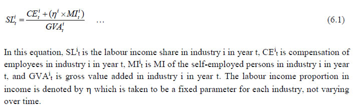 The derivation of the GVA series for different industries has been briefly explained in Chapter 2. The derivation of CE and MI series has been explained in step I above. Therefore, only the estimation method of ƞ needs to be described. The estimation of ƞ has been done with the help of NSS survey-based estimates of employment of different categories of workers (number of persons and days of work) and wage rates (which has been described briefly in chapter 4) coupled with estimates of MI, basically obtained from the NAS. Two approaches have been taken to get an estimate of ƞ, and the labour income share series for different industries finally adopted in the study makes use of an average of the estimates of ƞ obtained by the two approaches. In the first approach, an estimate of labour income of self-employed workers has been made for each study industry for five years, 1983-84, 1987-88, 1993-94, 1999-00, 2004-05, 2009-10, 2011-12 and 2015-16 on the basis of the estimated number of self-employed, wage rate of self-employed and the number of days of work per week. The industry-wise estimates of number of self-employed, wage rate of self-employed and the number of days of work per week have been made from unit records of NSS employment-unemployment survey (major rounds), as explained in chapter 4 above. The estimates of the number of self-employed, wage rate of self-employed and the number of days of work per week provide an estimate of the annual labour income of self-employed workers which is divided by the MI of self-employed (derived from NAS) to get an estimate of ƞ. For five industries, the ratio in question has been computed and applied. For the other 22 industries, the ratio in question has been computed after clubbing the industries into 11 industry groups.31 In the latter case, a common ratio computed for group of industries has then been applied to constituent industries. The list of industries or industry groups for which ƞ has been estimated is given in table 7.2. In the second approach, the NSS data are used to compute the following ratio: the ratio of labour income of self-employed workers to the labour income of regular and casual workers. Let this be denoted by θ. Then, the estimate of CE provided in the NAS is multiplied by θ to obtain an estimate of the labour income component out of the MI reported in the NAS. The labour component of MI divided by total MI gives an estimate of ƞ. In case the estimated labour component of MI exceeds the estimate of MI, the estimate of ƞ has been taken as unity. Examining the estimates obtained by the first approach, it was found that the estimated labour income share out of MI varied significantly among the estimates for the seven years for which the ratio in question has been estimated. The estimates of ƞ obtained by the second approach has the problem that in a number of cases, the estimated labour component of MI exceeds the estimate of MI given in the NAS, and therefore ƞ is taken as one. The method finally adopted is as follows: (a) The average value of ƞ has been computed for each industry or industry group by taking the estimates for the years 1983-84, 1987-88, 1993-94, 1999-00, 2004-05, 2009-10, 2011-12 and 2015-16. This has been done separately for the estimates based on approach-1 and those based on approach-2. (b) The estimates of ƞ obtained for each industry or industry group by the two approaches have then been averaged. (c) Having obtained an estimate of ƞ, equation 6.1 given above has been applied to compute the labour income share. b) Construction of Factor Income Share Series in Gross output The income share of labour, capital and intermediate inputs in Gross output has been computed using the following steps:
The splitting of unorganised sector factor incomes into individual industries has been done using unorganised survey results. The proportions computed for 1983-84 has been applied for the period 1980-81 to 1983-84. While there were surveys of unorganised manufacturing enterprises in 1978-79 the survey results have not been used for estimation of factor incomes in different industries of the unorganised manufacturing sector. Chapter 8: Growth Accounting Methodology This chapter deals with the methodology of measurement of total factor productivity (TFP) growth for individual industries in the KLEMS framework and the aggregation from industry level productivity measures to measures for broad sectors and the economy as a whole. The methodology of analysis of sources of gross output growth at the individual industry level and sources of Gross value added (GVA) or GDP growth at the broad sector level and economy level will also be presented in this chapter 8.1 Methodology for Measuring Productivity Growth at the Industry level The production function Our measurement of TFP growth for different industries of the Indian economy is based on a gross output production function for each industry j:  Y is industry gross output, L is labour input, K is capital input and E, M and S are intermediate inputs-namely energy, material and services and T is an indicator of technology for industry j. All variables are indexed by time (t subscript is suppressed). There are several things to note about the production function- (1) all variables are aggregates of many components that have been discussed in the earlier report/chapters; (2) we assume that the industry production function is separable in these aggregates; (3) time (indicator of technology) enters the production function symmetrically and directly with inputs. An important feature of the gross output approach is the explicit role of intermediate inputs. In our study, we have considered three intermediate inputs - energy, material and services and; this is important as we may find that intermediate inputs are the primary component of some industries outputs.32 Failure to quantify intermediate inputs leads us to miss both the role of key industries that produce intermediate inputs and the importance of intermediate inputs for the industries that use them. In order to estimate the production function at constant prices, the industry level price data is used for output, capital, labour and intermediate inputs, e.g., PYj; PLj, PKj; PEj. PMj, PSj. We assume that all industries face the same input prices. The industry price of an input varies across industries due to compositional effects as industries expend different shares of their investment on each type of asset. The same is true for all inputs. Total Factor Productivity To estimate TFP growth, we begin with the fundamental accounting identity for each industry where the value of output equals the value of inputs.  Under specific assumptions of constant returns to scale and competitive markets, we can define TFP growth as 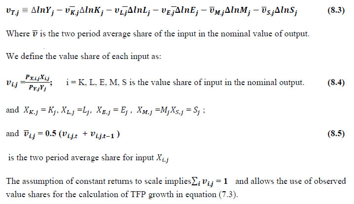 Rearranging equation (8.3), yields the standard growth accounting decomposition of output growth into the contribution of each input and the TFP residual  where the contribution of an input is defined as the product of the input’s growth rate and its two period average value share. We can further decompose the contribution of each input into a quantity and quality component. As discussed earlier, the quality component represents substitution between H components, while the quantity component represents the increases in each detailed input. Our extended decomposition of the sources of output growth is 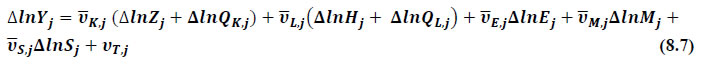 Where Z is the stock of industry capital, Qk is the capital quality, H is number of persons employed and Ql is the quality of labour. 8.2 Methodology for Aggregation across Industries In the analysis presented in the above section, gross value of output (GVO) is taken as the measure of output of an industry and TFP growth was estimated using the gross output function framework in which capital, labour, material, energy and services are taken as five inputs (in the case of agriculture, land was included among inputs). The Törnqvist index is applied to estimate TFP growth for each year during 1980-81 to 2016-17, which yielded an index of TFP for each industry for that period, permitting estimation of trend growth rate in TFP for the period under study (1980-81 to 2016-17). The method of estimation of TFP growth for individual industries described in section 8.1 cannot be readily applied to a higher level of aggregation. The main problem is that gross value of output cannot be added across industries to generate a measure of output at a higher level of aggregation, say for the economy or of any of the broad sectors. It becomes necessary therefore to consider appropriate methods of aggregation across industries consistent with the gross output function specification at the individual industry level. It is needless to say that one has to use the concept of value added to define an appropriate measure of output at the economy or broad sector level, but even here there are important issues of aggregation, i.e., how value added in different industries should be combined. A very useful discussion of the issues involved is found in Jorgenson et al., (2005). There are three approaches to estimating TFP growth at an aggregate level. This is discussed in detail in Jorgenson et al., (2005). The first approach is called aggregate production function approach. This approach assumes the existence of an aggregate production function (say, at the level of the economy or at the level of manufacturing or services sector). An essential condition is that the production function be separable in primary inputs. Let the production function for a particular industry be defined as:  where Y denotes gross output, X intermediate input (in turn a combination of materials, energy and services), K capital input, L labour input and T time (representing technology). Then, the concept of value added requires the existence of a value added function which in turn requires that the above production function be separable in K, L and T, i.e., the production function should take the following form:  In this equation, V (.) is the value added function. V denotes value added. Besides the condition of separability of the production function described above, a number of highly restrictive assumptions have to be made for the aggregate production function approach. These include: (a) the value added function is the same across all industries up to a scalar multiple, (b) the functions that aggregate heterogeneous types of labour and capital must be identical in all industries, and (c) each specific type of capital and labour receives the same price in all industries. With these assumptions made, real value added at the aggregate level becomes a simple addition of real value added in individual industries. In notation,  where Vi is value added in the ith industry and V is the aggregate value added. Given aggregate value added and somewhat similarly defined aggregate capital and labour input, TFP growth at the aggregate level can be computed. The second approach to aggregation is the aggregate production possibility frontier approach. It also needs the separability condition described in equations 8.8 and 8.9 above, as in the case of the aggregate production function approach. The main difference between the aggregate production function approach and the aggregate production possibility frontier approach is that the latter relaxes the assumption that all industries must face the same value added function. Thus, the price of value added is no longer assumed to be the same across industries. The implication is that the aggregate value added from the aggregate production possibility frontier is given by the Törnqvist index of the industry value added as:  In this equation, wi is the share of industry i in aggregate value added in nominal terms. Thus, defining PV,i as the price of value added in industry i and Vi as the real value added in industry i, the share in question may be defined as:  and the two period average is defined as:  Since each industry is subject to a production function separable in capital, labour and technology, as defined in equation 8.9, real gross output, real value of intermediate inputs and real value added of industry i in a particular year t should satisfy the following relationship:  In this equation, uV and uX are the shares of value added and intermediate inputs in the gross value of output in nominal terms. Given data on growth in gross output and growth in intermediate inputs of a particular industry, the above equation yields the growth in real value added of that industry. TFP growth from the aggregate production possibility frontier may be defined as follows:  In this equation K and L are aggregate capital input and labour input, respectively, and vK and vL are value shares (or income shares) of capital and labour, respectively. If one maintains the assumption that each specific type of capital and labour input has the same price in all industries, then each type of capital (labour) can be summed across industries and then a Törnqvist index can be constructed to yield aggregate capital (labour) input. Alternatively, different types of capital input can be combined using a Törnqvist index into total capital input used in an industry and then industry level growth in capital input can be combined with the help of a Törnqvist index to obtain growth in capital input at the aggregate level. In a similar manner, the growth in aggregate labour input can be computed. The third approach to measuring the TFP index at a higher level of aggregation is to apply direct aggregation to industry level estimates. This maintains the industry level production accounts as the fundamental building block and begins with industry level sources of growth. Of the three approaches described here, this is the least restrictive in terms of the assumptions involved. The following equation expresses the relationship between aggregate value added growth and the growth in capital and labour inputs and TFP in individual industries:  In this equation, vK is the value share of capital in gross output, vL is the value share of labour in gross output, vV is the share of value added in gross output, and wi is the share of industry i in aggregate value added in nominal terms. The bars indicate that the average of two periods, t and t-1, are to be taken. The last term in equation 8.16 is:  This is the Domar aggregation of TFP growth rates at individual industry level. Note that it is weighted average of industry level TFP growth rates. But, the weights add up to more than one. The data constructed for GVA and gross output, labour input, capital inputs, intermediate inputs and factor income shares (Chapters 2,3,4,5,6 and 7 respectively), are used to estimate TFPG during the period 1980 to 2016. Labour input is measured using total person worked (see, Chapter 4 for the detailed discussion). The series on growth rate in capital services is taken from Chapter 5. Chapter 9: Extension to KLEMS Variables A. Energy intensity series – note on data sources and computation methodology 9.1 Time period covered and level of disaggregation
9.2 Concepts and methods
Data on GVA and gross output
Data Sources on energy consumption
Conversion factors
Some adjustments made to official data
9.3 Deriving energy use estimates for manufacturing
B. Estimating aggregate economy ICT investment and Capital39 This section explains the approach used to estimate investment in ICT assets for the total economy. Investment in ICT is defined as investment in three asset types: hardware, communication equipment, and software. We first explain the construction of investment data for each of these asset types and subsequently explain the construction of capital stock and capital services. The primary source of data we rely on for these estimates is official national accounts data, input-output tables and World Information Technology and Services Alliance (WITSA)40’s estimates on ICT spending. Software investment: National Accounts Statistics provides software investment by different undertakings covering administrative departments, autonomous bodies, cooperatives, departmental enterprises, household sector, non-departmental enterprises, private corporate sector, and public administration, since 1999. We have obtained this data disaggregated by industries from the Central Statistics Office (CSO), and this has been the primary series we consider as the benchmark series of software investment for India. For years before 1999, we extrapolate software series by applying software/hardware ratio to measured series of hardware investment (measurement of hardware series is discussed below). We generate a series of software/hardware ratio using the trend in software/hardware ratio in the United States. The U.S data has been obtained from the EU KLEMS database.41 While this is a rough assumption, it is better than assuming a constant or linearly growing software/hardware ratio. The U.S, being the ICT leader, may provide a realistic picture of the required hardware/software ratio, particularly in the early years.42 Hardware investment: National Accounts provides a series on investment in ICT equipment since 2012. But it does not provide a split between hardware and communication equipment, which are often considered separately in the literature. Moreover, this data is not available for years before 2012, during which ICT equipment was part of total machinery investment. Therefore, in the India KLEMS approach, we estimate the hardware and communication equipment investments separately for years before 2012, and then club them into one category, ICT equipment, in order to keep consistency with the National Accounts data. In constructing a series of software investment, once hardware data is available, de Vries et al., (2010) suggest using the elasticity of hardware to software investment, estimated using a fixed effect panel regression of software on hardware and a set of control variables. We follow a similar approach to derive hardware investment, but not using econometric techniques. We use software/hardware ratio from WITSA ICT spending data. While doing this, we exclude consumer spending. This ratio is applied to software series obtained from National Accounts, thus providing us a hardware series for 1999-2011. For years before 1999, hardware series is obtained using the trends in the hardware investment series arrived at using a commodity flow approach (CFM)43. That is the benchmark series for 1999 is extrapolated using the annual changes in the investment series obtained using the CFM. In the CFM approach, total economy investment in hardware and communication equipment can be estimated using the information on the overall domestic availability of these goods and its investment component. This requires the use of input-output tables, in combination with NAS and trade statistics. We define the investment in ICT asset i as:  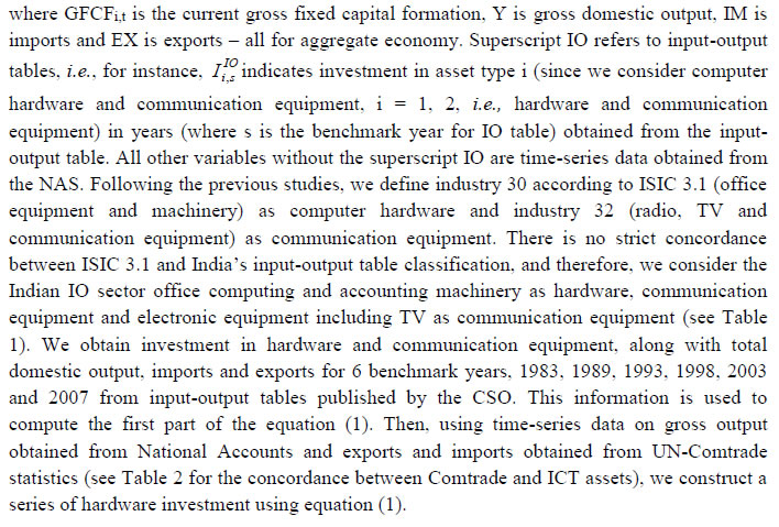 As mentioned before, to extrapolate hardware investment series backward we apply the trend in the obtained hardware series to 1999 hardware investment obtained using software/hardware ratio from WITSA applied to software data from NAS. Alternatively, one could directly take the series generated using commodity flow approach for the entire period (i.e., before and after 1999). However, we opted not to do so, because, the industry concordances are not at the maximum precision for IO tables after 2003. Hence, as discussed earlier, we constructed the hardware series for years after 1999 using NAS based software and WITSA based software/hardware ratio. Since the commodity flow approach produces a different estimate for hardware investment in 1999, to keep consistency, we proportionally adjust the series based on commodity flow approach – i.e., by applying the annual changes in commodity flow-based series to the 1999 benchmark estimate of hardware investment. Communication equipment: For the communication equipment series, we directly take the series generated using the commodity flow approach, using data from the IO table, because the industry description was entirely consistent and clear (see Table 1). Once the hardware and communication equipment investment data are obtained, we club these two to obtain total ICT equipment data. The trend in the estimated ICT equipment series is then applied to the published national accounts series on ICT equipment in 2012, to generate a consistent series for the earlier years. This way, we have a complete series of nominal values of ICT investment for the aggregate economy. This approach allows us to generate investment series only for the total economy, as an industry break-down is not possible with the input-output table. For the two assets, ICT equipment and Software, investment series for years before 1983 (i.e., the first benchmark I-O table), we linearly forecast the domestic availability ratios (see equation 1), until 1970. The investment estimates obtained from this linearly interpolated series will be used to derive initial capital stock (see section 5.2). ICT prices and depreciation To deflate the nominal investment series, in order to construct ICT capital stock, we also require price deflators of ICT assets. Price measurement for ICT assets has been an important research topic in the literature, as the quality of ICT capital goods has been rapidly increasing. The use of a single harmonized deflator across countries was widely advocated and used (Timmer and van Ark, 2005; Schreyer, 2002). We use a harmonization procedure suggested by Schreyer (2002) where the US hedonic deflators44 are adjusted for India’s domestic inflation rates, i.e., 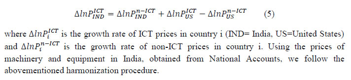 For the depreciation rates, following the standard practice in the literature. Jorgenson and Vu, (2005) assumes a 31.5 percent depreciation rate for software and hardware and 11.5 percent for communication equipment. Since we do not have the split between hardware and communication equipment in our data (except for the historical series from CFM), we use an average depreciation rate for hardware and communication, viz. 21.5 percent. ICT Capital stock As is the case with all other assets, we use a standard perpetual inventory method (PIM) to estimate ICT capital stock (See section 5.1). Capital stock for a given ICT asset i can be obtained using the PIM as: 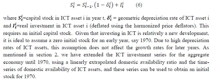 1 Timmer, M.P, Mahony, M. and van Ark, B. (2007). The EU KLEMS growth and productivity accounts: an overview. Mimeo University of Groningen & University of Birmingham, 2 Readers can refer to India KLEMS Data Manual Version 2013 for the data set released by RBI on its website in June 2014. 3 From both aggregated 9 NAS sectors Gross Domestic Product by economic activity statement along with the disaggregated statements of these 9 NAS sectors. 4 It uses NAS Series 2004-05 for more recent years. 5 Kanhaiya Singh and M.R. Saluja (2016), Input-Output Table for India, 2013-14, Working Paper no WP-111, National Council of Applied Economic Research, New Delhi 6 The principal components of Manufacturing n.e.c are manufacturing of jewellery and related articles, manufacture of musical instruments, manufacture of sports goods, manufacture of games and toys and other manufacturing. 7 See Himanshu (2011) for a discussion on many issues associated with the NSSO employment surveys. 8 The interpolation methodology and the use of other sources for few industries is explained in the subsequent section. 9 The coverage and the sample size of thin rounds is different from major rounds. 10 Problems in using UPSS are: The UPSS seeks to place as many persons as possible under the category of employed by assigning priority to work; no single long-term activity status for many as they move between statuses over a long period of one year, and Usual status requires a recall over a whole year of what the person did, which is not easy for those who take whatever work opportunities they can find over the year or have prolonged spells out of the labour force. 11 In EU-KLEMS changes in labour composition has been measured by including employment class, gender, age and education (Timmer, op cit; p64) and only 3 categories of education defined as high skilled, medium skilled and low skilled have been taken. This concept of labour composition is refereed as ‘labor quality’ by Jorgenson. It is recognized (Timmer; op cit; p84) that the categorization may lead to biases in the aggregate composition adjustment if employment trends and wage share differ within categories. These education categories generally correspond to- up to Primary education, above Primary to Higher Secondary education and above Higher Secondary or College education. Due to data limitations in India we have measured changes in labour composition only by changes in education profile of labour; hence named it labour education index. Therefore it became necessary to have a more detailed classification of education to capture the changes in skill composition of labour in India. For comparison, we estimated the changes in labour composition based on three education categories also and found that for the total economy the annual trend growth in labour education index is 1.16 per cent as compared to 1.25 per cent based on five education categories. 12 This procedure has been advocated by NSSO itself and has been consistently adopted by almost all researchers. 13 A very lucid description of the same is given by Sivasubramonian (2004). 14 Appendix Table D provides the details about the Census Population, WFPR by UPSS, and persons employed in each of the EUS rounds used in the study. 15 The 66th round has not been used because of its inconsistency with the 61st and 68th round. Most economists consider it as an outlier. 16 Since 2009-10, the labour Bureau, GOI has started collecting annual data on Employment and Unemployment and has released five reports till 2015-16. Its estimates are not comparable with EUS and the unit level data, which is used to get employment by different characteristics-age, gender, education, etc. is also not provided. So only the growth rates provided by Labour Bureau data are used in the KLEMS employment series. 17 Aggregate input is measured as a translog index of its individual components. Then the corresponding index is a Törnqvist volume index (see Jorgenson, Gollop and Fraumeni 1987). For all aggregation of quantities we use the Törnqvist quantity index, which is a discrete time approximation to a Divisia index. This aggregation approach uses annual moving weights based on averages of adjacent points in time. The advantage of the Törnqvist index is that it belongs to the preferred class of superlative indices (Diewert 1976). Moreover, it exactly replicates a translog model which is highly flexible, that is, a model where the aggregate is a linear and quadratic function of the components and time. 18 Although census population is available only decennially, we used the interpolated population figures for the mid-year survey periods [Visaria, (1996) for 1977-78 (Jan) and 1987-88 (Jan); Sundaram, (2007) for 1983 (July), 1993-94 (Jan), 1999-00 (Jan) and 2004-05 (Jan)] and from NSSO (2010) for Jan 2010 and Jan 2012. 19 In EU KLEMS (Timmer, op cit; p 67) it is assumed that the earnings is equal to the earnings of ‘regular' employees. 20 The details of the function can be obtained from the Stata software and from Appendix. 21 Asset prices are used in the aggregation of capital stock. However, it is the price of the capital service that must be used in aggregating capital services (see Jorgenson and Griliches, 1967; Diewert, 1980) as it is the services delivered by capital goods that are used in the production process. Jorgenson and Griliches (1967) have shown that these two prices are related; the asset prices are the discounted value of all future capital services. They are not proportional though, as there are differences in replacement rates and capital gains among different capital assets. 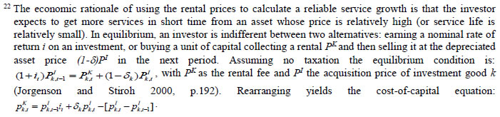 23 This version of the database does not make a distinction between ICT and non-ICT assets, as the industry level data on ICT assets are weak. An attempt to estimate aggregate economy level ICT capital can be found in Erumban and Das (2015). 24 See O’Mahony and Timmer (2009) for a description of EU KLEMS database 25 This data is not publicly available. However, CSO has been kind to compile this data for the India-KLEMS project. 26 In some years transport equipment was provided as part of the machinery and equipment, categorized as ‘tools, transport equipment and other fixed assets’. In such cases, we use transport/tools, transport and other fixed asset ratio in the nearest year to separate transport equipment. 27 This choice is driven by the fact that the first year of availability of ASI data is 1964-65. 28 National Accounts Statistics-Sources and Methods, Chapter 26, CSO (2007) 29 We do not intend to delve into the controversies over the use of internal vs. external rate of return in the context of productivity measurement. Rather, given that this is the first version of our data, we use the external rate and in a later stage, we will also use internal rates. See Erumban (2008a and b) for a discussion on these issues. 30 Reserve Bank of India, Handbook of Indian Statistics, Annual volumes. 31 The estimation is done at group level rather than individual industries on the consideration that the group level estimates will be more reliable. 32 Consider, the semi-conductor (SC) industry, which is a key input to the computer hardware industry. Much of the output is invisible at the aggregate level because semi-conductor products are intermediate inputs to other industries rather than deliverables to final demand - consumption and investment goods. Moreover, SC plays a role in the improvements in quality and performance of other products like - computers, communication equipment and scientific instruments. Failure to account for them leads us to miss the role of key industries that produce intermediate inputs and importance of intermediate inputs for the industries that use them. (Jorgenson, Ho and Stiroh (2005), Productivity, volume 3). 33 Sectoral break-up of consumption of lubricants is not available. It has been assumed that two-thirds is used in industry and one-third in transport. There is a small part being used by tractors in the agriculture sector. This is ignored. The basis for the above assumption is the estimates of consumption presented in a recent report available on the internet (Sabri Hazarika, India’s Lubricants Sector, The Road to Recovery, Philip Capital India Research, available on line at: http://backoffice.phillipcapital.in/Backoffice/Researchfiles/PC_-_Indian_Lubricants_Sector_-_Sep_2016_20160920081315.pdf, accessed on 31 March 2019). For motor spirit, it is assumed that 75 per cent is consumed by households and 25 per cent by the transport sector. The basis for this assumption is break-up of petrol consumption by type of vehicle available for 2012-13 in a report of the Petroleum Planning and Analysis Cell (All-India Study on Sectoral Demand of Diesel and Petrol, Report, Petroleum Planning and Analysis Cell, Ministry of Petroleum and Natural Gas, Government of India, 2013). 34 These energy intensity series (being based on quantum of energy use in physical units) are different from energy intensity that can be computed by dividing deflated value of energy input by real value of gross output available in the India KLEMS database. The latter series has certain limitations. For instance, if power is supplied to agriculture free of cost, this will be captured properly if energy use is measured in physical unit, but not when the cost incurred on energy is considered. 35 Press note on National Accounts Statistics Back-series 2004-05 to 2011-12, base 2011-12, Central Statistics Office, Ministry of Statistics & Programme Implementation, Government of India, dated 28 November 2018. 36 This is based on calorific value of non-coking coal as given in India’s second Biennial Update Report to the UNFCCC (United Nations Framework Convention on Climate Change), December 2018, available on line at: https://unfccc.int/sites/default/files/resource/INDIA%20SECOND%20BUR%20High%20Res.pdf, accessed on 31 March 2019. The calorific value of coal used for power generation is lower than the calorific value of coal used in manufacturing. 37 All-India Study on Sectoral Demand of Diesel and Petrol, Report, Petroleum Planning and Analysis Cell, Ministry of Petroleum and Natural Gas, Government of India, 2013. According to this survey, 13 per cent of diesel is used by the agriculture sector. A working paper of NIPFP (Mukesh Anand, “Direct and Indirect use of Fossil Fuels in Farming: Cost of Fuel-price Rise for Indian Agriculture,” Working paper no. 2014-132, National Institute of Public Finance and Policy, New Delhi, 2014) reports that the share of agriculture in total diesel consumption was 19.2 per cent in 1998-99, 19.8 per cent in 2000-01, 11.9 per cent in 2008-09 and 12.2 per cent in 2010-11. 38 Sudhir Gota, “Transport Emissions and India’s Diesel Mystery Comparing Top-Down and Bottom-Up Carbon Estimates.” Working Paper. Washington, DC: EMBARQ. 2014. Available online at: http://www.embarq.org/our-work/research; Nan Zhou and Michael A. McNeil, “Assessment of historic trend in mobility and energy use in India transportation sector using bottom-up approach.” Journal of Renewable and Sustainable Energy 1(4), 2009. 39 The discussion in this section on aggregate economy ICT investment heavily draws upon Erumban and Das (2016). 40 WITSA provides ICT spending data in a cross section of countries through their Digital Planet Report. See http://www.witsa.org/ 41 We use the 2011 version of the EU KLEMS data, see www.euklems.net. 42 Note that the software investment data – be it directly from the NAS, or obtained using hardware/software ratio from WITSA or from the United States - does not capture pirated software used by companies, if any. While the use of such pirated software would indeed contribute to firm’s output growth, it will never be reported by firms, and hence is hard to capture. 43 See de Vries et al., (2010) and Timmer and van Ark (2005) for a good description of the commodity flow approach. 44 Our harmonized price deflators are based on the U.S hedonic prices, which are constructed using a hedonic regression where prices of ICT equipment regressed on several characteristics, such as for instance processor speed, hardware size, memory etc. |
|||||||||||||||||||||||||||||||||||
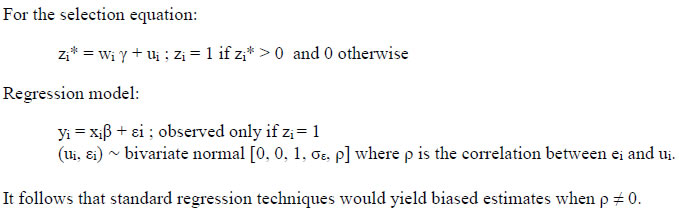
Measuring Productivity at the Industry Level - The India KLEMS Database
|
AUTHORS Deb Kusum Das Abdul Azeez Erumban Suresh Aggarwal Pilu Chandra Das
Changes in India KLEMS Database 2020 over the India KLEMS Database 2019 version Overall changes The database is extended to include 2018-19 for all variables, thus providing a series for the period 1980-81 to 2018-19 Variable specific changes 1. Gross Value Added Estimates of Gross Value Added (GVA) for years since 2011-12, both current and constant (2011-12) prices for all industries are obtained from National Accounts Statistics (NAS) 2021. 2. Gross value of Output Estimates of Gross Value of Output (GVO) for years since 2011-12, both current and constant (2011-12) prices for all industries are obtained from National Accounts Statistics (NAS) 2021. 3. Labour Input The latest Periodic Labour Force Survey (PLFS) by NSSO for 2018-19 on employment is used for estimating employment for 2018-19. 4. Capital Input
This document describes the procedures, methodologies and approaches used in constructing the India KLEMS database version 2020. This database is part of a research project, supported by the Reserve Bank of India (RBI), to analyze productivity performance in the Indian economy at disaggregate industry level. This work is meant to support empirical research in the area of economic growth. In addition, the database is meant to support the conduct of policies aimed at supporting acceleration of productivity growth in the Indian economy, requiring comprehensive measurement tools to monitor and evaluate progress. Finally, the construction of the database would also support the systematic production of reliable statistics on growth and productivity using the methodologies of national accounts and input-output analysis. In its definitive version the India KLEMS research project will include measures of economic growth, employment creation, capital formation and productivity at the industry level from 1980-81 onwards. The input measures will incorporate various categories of Capital (K), Labour (L), Energy (E), Materials (M) and Services (S) inputs. A major advantage of growth accounts is that it is embedded in a clear analytical framework rooted in production functions and the theory of economic growth. It provides a conceptual framework within which the interaction between variables can be analyzed, which is of fundamental importance for policy evaluation (Timmer et.al.2007)1. The present document describes the India KLEMS database version 2020. The present version is an extended India KLEMS research project, “Disaggregate Industry Level Productivity Analysis for India- the KLEMS Approach” being undertaken at the Centre for Development Economics, Delhi School of Economics. This one builds on the previous project, which was undertaken at ICRIER, New Delhi2. The Data Manual is intended to guide researchers about the variables (and their construction) used to measure both inputs and total factor productivity (TFP) at the industry level using the dataset. In addition, it is also intended to support national officials’ statistical agencies in future work on the productivity database within the agencies. The dataset includes measures of Gross Value Added (GVA), Gross Value of Output (GVO), Labour (L), Capital (K), Energy (E), Material (M), Services (S), Labour Quality (LQ), Labour Productivity (LP) and Total Factor Productivity (TFP) at the industry and economy level from 1980-81 onwards. The database covering the period 1980-81 to 2018-19 has been constructed on the basis of data compiled from CSO, NSSO, ASI, Input-Output tables (I-O tables) and processed according to appropriate procedures. These procedures were developed to ensure harmonization of the basic data, and to generate growth accounts in a consistent and uniform way. Harmonization of the basic data has focused on a number of areas such as industrial classification, and aggregation levels. The data base covers 27 industries comprising the entire Indian economy. The industries are shown in Table 1.1 below. The variables in the data set are given in Table 1.2. 1.2 Coverage: Industries and Variables In this section we describe the coverage of the India KLEMS database in terms of industries and variables. In principle, the 39-year period from 1980-81 (1980) to 2018-19 (2018) is covered. At a disaggregated level, database is created for 27 industries. The industrial classification is constructed by building concordance between NIC 2008, NIC 2004, NIC 1998, NIC 1987 and NIC 1970 so as to generate continuous time series from 1980 to 2018. This classification is very close to the International Standard Industrial Classification (ISIC) revision 3. The 27 industries are aggregated to form six broad sectors, namely:
Table 1.1 provides a listing of the 27 industries, including the higher aggregates. Further the detailed classification and concordance of study industries with NICs is provided in Appendix table A. Table 1.2 provides an overview of all the series included in our database. Measures of Capital (K), Labour (L), Energy (E), Material (M) and Service (S) inputs as well as Gross Output (GO), have been constructed using National Accounts Statistics (NAS), Annual Survey of Industries (ASI), NSSO rounds and Input-Output Tables (IO). In building annual time series on gross output, five inputs and factor income shares, various assumptions are made to fill up gaps in industry details and link series over time. As we know that NSSO rounds of unregistered manufacturing, Input Output Transaction Tables, and Employment and Unemployment Surveys by NSSO are available only for certain benchmark years. Thus, the use of information from these data sources necessitates interpolation and assumption of constant shares for building series of output and inputs. The construction of growth accounting series like total factor productivity, labour productivity are based on theoretical models of production and needs additional assumptions that are spelt out in subsequent chapters of the manual. Finally, the other Series like NDP at factor cost, compensation of employees etc. are additional series which are used in generating the growth accounts and are informative by themselves. Chapter 2: Gross Value-Added Series at the Industry Level For an individual firm or industry, productivity measure can be based on a value-added concept where value added is considered as an industry’s output and only primary inputs such as labour and capital are considered as industry inputs. Value added based productivity measures reflect an industry’s capacity to contribute to economy-wide income and final demand. In this sense, they are valid complements to gross output-based measures. This chapter describes the data sources and methodology used to construct the Gross Value Added (GVA) series at current and constant prices for 27 study industries for the period of 1980-81 (1980) to 2018-19 (2018). GVA of a sector is defined as the value of output less the value of its intermediary inputs. This value added created by a sector is shared among the primary factors of production, labour and capital. The National Accounts Statistics (NAS) brought out by the CSO (Central Statistics Office, Government of India) is the basic source of data for the construction of series on gross value added for INDIA KLEMS-industries. NAS provides estimates of GVA (i.e., gross value added) at a disaggregated industry level at both current and constant prices for the period since 1950-51. Up to 2011-12, estimates of GVA at both current and constant (2011-12) prices for all industries are obtained from Back Series of National Accounts (Base 2011-12). For years after 2011-12, they are directly obtained from NAS 2021. However, NAS estimates of value added are not available for a few India KLEMS industry groups. Therefore, we had to split some of the aggregate industry groups from NAS. In the previous versions of the India KLEMS data, value-added was measured at factor cost (as was the case with the NAS). However, this was not fully consistent with the KLEMS standards used internationally, as the international standards of KLEMS methodology were to follow value added at basic prices.3 Our choice to use the factor price concept was driven by the fact that the NAS provided gross value added at current and constant prices only at factor cost. Since 2011-2012, following the SNA, the NAS started providing value added at basic prices, which we could directly use and keep the India KLEMS approach consistent with the general KLEMS standards. Therefore, the new version of the India KLEMS database bypasses the inconsistency with the KLEMS standards we had while maintaining consistency with the NAS, as the NAS has now entirely shifted to the basic price concept. NAS provides separate estimates of GVA for registered and unregistered manufacturing. However, onwards 2011-12 NAS has disaggregated the manufacturing sector in to corporate sector and household sector. For splitting the aggregate estimates of GVA for registered manufacturing industries and the corporate sector, we have used data from the Annual Survey of Industries (ASI) based on the National Industrial Classification 2004 and 2008 (NIC-2004 & NIC-2008). Whereas, for the unregistered manufacturing sector, we have used results from six rounds of NSSO surveys- [40th (1984-85), 45th round (1989-90), 51st round (1994-95) 56th round (2000-01), 62nd round (2005-06), 67th round (2010-11) and 73rd round (2015-16)] to obtain the value-added estimates. In India, GDP for unregistered manufacturing is constructed using the labour input method. The estimates of GVA for the unregistered manufacturing sector are obtained as a product of the workforce and the corresponding GVA per worker. The information about employment in the unorganized sector is only available in the benchmark years for which NSSO survey data are available. Therefore, there is no consistent source of employment data for the years between these quinquennial surveys. Even the information on value added per worker is equally limited since the value-added data are also updated on an approximate 5-year interval (for details, see CSO, 2007). Therefore, estimates of value added for the unregistered manufacturing sectors for the years between the benchmarks have been obtained by interpolation and for years outside the benchmark years by linear extrapolation. For splitting the aggregate estimates of GVA for the household sector for recent years (i.e., 2011 onwards), we have used GVA data from 67th round (2010-11) and 73rd round (2015-16). The construction of Gross valued added series involves three steps. Step 1: A concordance table between the classification used in the NAS and the 27 study industry classification used for this project has been prepared. Further, concordance between all the 27 sectors has been constructed with NIC- 1970, 1987, 1998, 2004 and 2008. Out of the 27 study industries, for 20 industries, GVA series both in current and constant prices is directly available from NAS4. The sectors for which data are provided in NAS are Agriculture, Forestry & logging, Fishing, Mining and Quarrying, Manufacturing (registered and un-registered), Electricity, Construction, Trade, Hotels & Restaurants, Railways, Transport by other means, Storage, Communication, Banking & insurance, Real estate, Ownership of Dwelling & Business Services, Pubic Administration & Defense and Other Services. Step 2: For manufacturing industries where direct estimates of GVA were not available from NAS, estimates have been made using additional information from ASI and NSSO unorganized manufacturing data. GVA data are directly available from NAS for 6 out of 13 manufacturing sectors the period 1980-81 to 2011-12, while for 8 out of 13 manufacturing sectors GVA data directly available since 2011-12. The list of these industries is provided in the table below. For the remaining industries GVA data is constructed by splitting the NAS data using ASI or NSSO distributions. ASI data (annual) has been used for registered manufacturing whereas interpolated ratios from NSSO 40th (1984-85), 45th (1989-90), 51st (1994-95), 56th (2000-01) 62nd (2005-06), 67th round (2010-11) and 73rd round (2015-16) rounds have been used for Unregistered Manufacturing segments. A list of study industries is presented in Table 2.2 and 2.3 showcasing the methodology used to split GVA of certain NAS sectors to match concordance with our classification. Following are the details of steps taken in splitting NAS sectors into India KLEMS industries for which direct Gross Value Added series are not available between 1980 and 2011. Wood and wood products and manufacturing of furniture In India KLEMS the sectors Wood products (20) and Furniture and fixtures (361) are considered separately, with the latter being added to the sector Manufacturing nec and Recycling (36+37). These sectors are available separately since 2011-12 from National Accounts (NAS 2021). However, the Back Series of National Accounts (Base 2011-12) does not provide them separately; rather it provides the data for the aggregate sector Wood and Wood products, furniture, fixtures etc. (20+361) – both for registered and unregistered sectors. For the registered segment of the industry, we split the value added in this aggregate sector to two individual sectors using the share of the respective sectors from the Annual Survey of Industries (ASI). For the unorganized segment, we use the shares of the respective sectors obtained from NSSO unorganized manufacturing surveys of the benchmark years (1984-85, 1989-90, 1994-95, 2000-01, 2005-06 and 2010-11), to split the aggregate data. The shares for the interim years between two benchmark years have been linearly interpolated till 2011-12, and for the period 1980-81 to 1984-85, the share of 1984-85 has been used. Coke, Refined Petroleum Products and Nuclear Fuel and Rubber and Plastic Products We split ‘Rubber, Petroleum Products’ (which are clubbed under one group in NAS) to arrive at two industry groups i.e., Coke, Refined Petroleum Products and Nuclear Fuel (23) and Rubber and Plastic Products (25). For the organized segment, we use the ASI (annual) data to get the individual sector shares and split the NAS data using these individual shares. Likewise, we use the relevant data from the four NSS surveys mentioned earlier to get the individual sector shares for the unorganized segment of this sector. The ratio of GVA for the interim years between two benchmark years have been linearly interpolated till 2011-12, and from 1980-81 to 1984-85, the ratio of 1984-85 has been used. Basic Metals and Fabricated Metal Products In our industry classification, Basic Metals and Fabricated Metal products (27+28) and Machinery (29) are separate groups whereas ‘Fabricated Metal Products’ (28); ‘Machinery and Equipment nec’ (29) and ‘Office, Accounting and Computing Machinery’ (30) are clubbed together as Metal Products and Machinery (28, 29 and 30) in NAS. To arrive at individual industry result, we use ASI shares for organized sectors and NSSO surveys for the unorganized sector. We add to the fraction of fabricated metal products (28) from Metal Products and Machinery to basic metals (271+272+2731 +2732) already available. Electrical and Optical Equipment In our study classification, ‘Electrical and Optical equipment’ includes all sectors from 30 to 33 under NIC 1998. However, ‘Electrical Machinery’ in NAS includes industries ‘Electrical Machinery and Apparatus n.e.c.’ (31) + ‘Radio, Television and Communication Equipment and Apparatus’ (32) and excludes ‘Office, Accounting and Computing Machinery’ (30) and ‘Medical, Precision and Optical Instruments’ (33). However, 30 is part of ‘Metal Products and Machinery’ and 33 is part of ‘Other Manufacturing’ in NAS. We take out 28 from Metal Products and Machinery in NAS, with 29 and 30 being left, which we split using ASI. NSSO surveys have been useful here as well to compute the unorganized segment share. Likewise, we also take out the share of 33 from ‘Other Manufacturing’ in NAS separately for both organized and unorganized segments to arrive at gross value added for electrical and optical equipment. NAS provides estimates of GVA for more disaggregate industries at both current and constant prices for the period since 2011-12. For 8 out of 13 manufacturing sectors GVA data are directly available from NAS. For the remaining 5 industries GVA data is constructed by splitting the NAS data using ASI or NSSO distributions. Following are the details of steps taken in splitting NAS sectors into India KLEMS industries for which direct Gross Value Added series are not available since 2011-12. Basic Metals and Fabricated Metal Products In our industry classification, Manufacture of structural metal products, tanks, reservoirs and steam generators (251) and Manufacture of other fabricated metal products; metalworking service activities (259) are combined as ‘Fabricated Metal Products’ (251+259) and Manufacture of weapons and ammunition (252) included in ‘Machinery nec’ whereas 251, 252 and 259 are clubbed together as Manufacture of fabricated metal products, except machinery and equipment (25) in NAS. To arrive at individual industry result, we use ASI shares for organized sectors and NSSO surveys for the unorganized sector. We add to the fraction of fabricated metal products (251 & 259) to basic metals (241+242+2431+2432) already available. Machinery, nec. In our study classification, ‘Machinery, nec.’ Includes 28, 252, 275, 304, 3311 and 3312 under NIC 2008. However, in NAS, Manufacture of fabricated metal products, except machinery and equipment (25) includes Manufacture of weapons and ammunition (252), Manufacture of electrical equipment (27) includes Manufacture of domestic appliances (275), Manufacture of transport equipment (29+30) includes Manufacture of military fighting vehicles (304), Repair and installation of machinery and equipment (33) includes Repair of machinery (3311 & 3312). We take out the required portion, which we split using ASI & NSSO ratio and added to already available Manufacture of machinery and equipment n.e.c. (28). Electrical and Optical Equipment In our study classification, ‘Electrical and Optical equipment’ includes 26, 27-275, 325, 3313, 3314, 3319, 3320 under NIC 2008. Using ASI and NSSO portion, we excluded the unrequired portion Manufacture of domestic appliances (275) from Manufacture of electrical equipment (27), and take out the required portion Manufacture of medical and dental instruments and supplies (325) from Other manufacturing (32) and Repair of electronic and optical equipment, electrical equipment and other equipment (3313, 3314, 3319 & 3320) from Repair and installation of machinery and equipment (33). Transport Equipment We excluded ‘Manufacture of military fighting vehicles (304) from Manufacture of transport equipment (29+30) and included Repair of transport equipment (3315) to arrive at industry group - Transport Equipment. It is important to note that the industry level value added volume indices are based on NAS. CSO provides single deflated value-added estimates for all sectors except Agriculture. Step 3: According to India KLEMS, output is adjusted for Financial Intermediation Services Indirectly Measured (FISIM). The value of such services forms a part of the income originating in the banking and insurance sector and, as such, is deducted from the GVA. The NAS provides output net of FISIM for some industry groups at a more aggregate level. For instance, in the estimates of GVA obtained for the registered manufacturing sector, adjustment for FISIM in NAS is made only at the aggregate level in the absence of adequate details at a disaggregate level. However, we have allocated FISIM to all the sectors of manufacturing by redistributing total FISIM across sectors proportional to their sectoral GDP shares. Similar redistribution of FISIM has been done in case of Real Estate, Ownership of Dwellings and Professional Services; and Other Services sector. Chapter 3: Gross Output Series at the Industry Level This chapter describes the procedures and methodologies used in constructing the database for gross output series at the industry level over the period 1980-81(1980) to 2018-19(2018). We discuss both the raw data sources and the adjustments that have been made to generate the time series on output and value added consistent with the official National Accounts. The methodology for measuring industry output, and value added was developed by Jorgenson, Gallop and Fraumeni (1987) and extended by Jorgenson (1990 a). Following a similar approach as explained in Jorgenson et al. (2005, Chapter 4) and Timmer et al. (2010, Chapter 3), the time series on gross output and intermediate inputs for the Indian economy have been constructed. The gross output of an industry is defined as the value of industry production using primary factors like labour, capital and intermediate inputs purchased from other industries. The gross output production function assumes separability in inputs and technology. An important advantage of the gross output approach is that it provides a complete measure of production and treats all inputs - labour, capital and intermediate inputs symmetrically. In contrast, the value-added measure of output does not explicitly account for the flow of intermediate inputs which may be the primary component of an industry’s output. We use the more restrictive value-added concept primarily because it is useful for aggregation purposes. It is to be noted that aggregate output (aggregated over industry value added), is a value-added concept and the detailed methodology of aggregation of output across industries is explained in chapter 8. To construct the gross output series at industry level, we use multiple data sources namely National Accounts Statistics, Annual Survey of Industries, NSSO rounds for unorganized manufacturing and Input Output Transaction tables. The data source and methodology used are documented below: National Accounts Statistics: The NAS is the basic source of data for the construction of time series on the gross output. The NAS back series 2011 with base 2004-05 and NAS 2014 provides estimates of gross output for six disaggregate industries at current and constant prices since 1950-51 till 2011-12. These sectors are Agriculture, Mining and Quarrying, Construction and Manufacturing sectors (Registered and Unregistered Manufacturing). However, the Back Series with base 2011-12, which is the source of GVA in India KLEMS database 2020, does not provide estimates of GVO for most of the industries except for Agriculture, Mining and Quarrying and Construction. For these three industries GVO data at current and constant prices directly obtained from Back Series with base 2011-12. Therefore, for 1980-81 to 2011-12 period, we estimate the GVO series for remaining 24 industries at current and constant prices by applying the respective GVO/GVA ratio for current and constant prices obtained from Back Series with base 2004-05 and NAS 2014 to GVA with 2011-12 base. For years since 2011, we take the estimates of GVO both at current and constant prices for all industries directly from NAS 2021. (a) Filling procedures of National Accounts series: It is to be noted that the NAS estimates of gross output for a few industry groups are at a more aggregate level, requiring splitting of the aggregates. In such cases, NAS estimates of output have been split using additional information from Annual Survey of Industries and NSSO rounds of Unregistered Manufacturing to obtain estimates at higher level of disaggregation. Secondly, for Unregistered manufacturing gross output data is available in NAS from 2004-05 onwards. In this case, information from NSSO survey rounds has been used for missing years to derive output estimates of unregistered manufacturing industries at current and constant prices. Annual Survey of Industries and NSSO Quinquennial Survey Reports: As mentioned above, gross output data are available at a more disaggregated level in Annual Survey of Industries (ASI) and NSSO quinquennial surveys for Registered and Unregistered Manufacturing industries, respectively. These secondary data sources are used in this study for two purposes: (a) in certain cases NAS provides combined estimates of GVO and GVA for two manufacturing industries. In such cases separate estimates for individual study industries are obtained with the help of ASI or NSSO unorganized manufacturing sector data. (b) For the period prior to 2004, NAS does not provide estimates of GVO for unorganized manufacturing industries. To make our estimate of GVO for this period, the NSSO data are used. The Major NSSO Rounds for Unregistered Manufacturing used are 40th Round (1984-85), 45th Round (1989-90) and 51st Round (1994-95), 56th Round (2000-01), 62nd Round (2005-06), 67th Round (2010-11) and 73rd Round (2015-16). Input Output Transaction Tables: As motioned earlier, for gross value-added series of service sectors we obtain our estimates from NAS. However, prior to 2011-12 National Accounts do not provide any estimates of gross output of service sectors and hence we rely on Input output transaction tables which are available at an interval of 5 years or so. This necessitates interpolation and assumption of constant shares for measuring output of services sectors. The Input Output Transaction Tables for Benchmark years of 1978-79, 1983-84, 1989-90, 1993-94, 1998-99, 2003-04 and 2007-08 are used to derive gross output series for service sectors. The construction of the gross output series from 1980 to 2017 at current and constant prices involves the following steps: Step 1: Measuring Gross Output of Agricultural Sector, of Mining and Quarrying, and Construction NAS provides nominal and real GVO series for a) Crops and Plantation, b) Animal Husbandry c) Forestry and Logging d) Fishing. By aggregating the GVO of these four subsectors we derive the GVO of Agricultural sector. The Gross output estimates of Mining and Quarrying and Construction at current and constant prices from 1980-2018 is also directly taken from NAS. Step 2: Measuring Gross Output of Manufacturing Industries For manufacturing industries time series on gross output is obtained by adding the magnitudes for registered and unregistered segments of manufacturing. As mentioned earlier, NAS estimates of gross output for manufacturing industries are at a more aggregate level. In such cases the aggregate output of NAS at current prices has been split using additional information from ASI and NSSO unorganized sector reports. Since 2011-12, gross output data for 8 out of 13 manufacturing industries listed in table 3.1 are directly picked up from NAS. For the remaining 5 sectors output is constructed by splitting the NAS output data using ASI or NSSO distributions. ASI data (annual) has been used for registered manufacturing whereas interpolated ratios from 67th (2010-11) and 73rd (2015-16) rounds have been used for Unregistered Manufacturing segments. A list of study industries is presented in Table 3.2 showcasing the methodology used to split GVO of certain NAS sectors to match concordance with our classification for the year 2011 to 2018. The detailed method of splitting the output of NAS sectors to derive output of individual industries is given as follows: Basic Metals and Fabricated Metal Products In our industry classification, Manufacture of structural metal products, tanks, reservoirs and steam generators (251) and Manufacture of other fabricated metal products; metalworking service activities (259) are combined as ‘Fabricated Metal Products’ (251+259) and Manufacture of weapons and ammunition (252) included in ‘Machinery nec’ whereas 251, 252 and 259 are clubbed together as Manufacture of fabricated metal products, except machinery and equipment (25) in NAS. To arrive at individual industry result, we use ASI shares for organized sectors and NSSO surveys for the unorganized sector. We add to the fraction of fabricated metal products (251 & 259) to basic metals (241+242+2431+2432) already available. Machinery, nec. In our study classification, ‘Machinery, nec.’ Includes 28, 252, 275, 304, 3311 and 3312 under NIC 2008. However, in NAS, Manufacture of fabricated metal products, except machinery and equipment (25) includes Manufacture of weapons and ammunition (252), Manufacture of electrical equipment (27) includes Manufacture of domestic appliances (275), Manufacture of transport equipment (29+30) includes Manufacture of military fighting vehicles (304), Repair and installation of machinery and equipment (33) includes Repair of machinery (3311 & 3312). We take out the required portion, which we split using ASI & NSSO ratio and added to already available Manufacture of machinery and equipment n.e.c (28). Electrical and Optical Equipment In our study classification, ‘Electrical and Optical equipment’ includes 26, 27-275, 325, 3313, 3314, 3319, 3320 under NIC 2008. Using ASI and NSSO portion, we excluded the unrequired portion Manufacture of domestic appliances (275) from Manufacture of electrical equipment (27), and take out the required portion Manufacture of medical and dental instruments and supplies (325) from Other manufacturing (32) and Repair of electronic and optical equipment, electrical equipment and other equipment (3313, 3314, 3319 & 3320) from Repair and installation of machinery and equipment (33). Transport Equipment We excluded ‘Manufacture of military fighting vehicles (304) from Manufacture of transport equipment (29+30) and included Repair of transport equipment (3315) to arrive at industry group - Transport Equipment. The nominal estimates of output for manufacturing sectors are then deflated with suitable WPI deflators to arrive at the constant price series. Step 3: Measuring Gross Output for Services Sectors and Electricity, Gas and water supply Onwards 2011 -12 NAS provided estimates of GVO at current and constant prices. Prior to 2011-12 Gross Output series for Services sectors and sector Electricity, Gas and Water supply has been constructed using information from Input – Output Transaction Tables of the Indian economy published by CSO.
Firstly, the present study provides estimates for manufacturing and its sub branches without segregating manufacturing (and its sub branches) into organized and unorganized segments. However, given the employment potential and sizable presence of the unorganized segment in many of the manufacturing industries, it would be worthwhile in Indian context to examine separately the productivity performances of both the organized and unorganized components. Some work to construct the output and input series separately for organized and unorganized components of Indian manufacturing has been done. A paper based on this analysis has been prepared. The data series for organized and unorganized manufacturing is not included in this release of India KLEMS database. Finally, National Accounts do not provide any estimates of gross output of services sector and hence we rely on Input output transaction tables which are available at an interval of about 5 years. This necessitates interpolation and assumption of constant shares for measuring output of services sectors. This issue is analogous to those explained in Timmer et al. (2010, Chapter 3) for the EU economy. Griliches (1994) paid particular attention to service sector output as a key source of uncertainty. Chapter 4: Labour Input Series at the Industry Level This chapter provides information on the sources of data and method of measuring labour services. The aim is to estimate labour input so that it reflects the actual changes in the quantity (number of persons) and quality of labour input over time. The section discusses the construction of labour input for 27 industries from 1980 to 2018. Labour input is measured by combining data on labour persons and data on labour quality. In the KLEMS framework it is desirable to estimate changes in labour quality by industries on the basis of age, gender and education. The measurement of labour quality is essentially an attempt to distinguish one labour type from the other taking into account the embodied human capital in each person. The source of human capital could be through investment in education, experience, training, etc. The contribution to output by each person also comes from this embodied capital and the reward (wages and earnings) to each person also includes the reward for investment in human capital. Therefore, it is essential to separate out these differences in labour to clearly understand the underlying differences in labour characteristics. It is in this context that an endeavor has been made to estimate labour quality index. Nevertheless, many limitations of India’s employment statistics, especially the availability of information on wages/ earnings of different category of workers which could be used as an indication of their differences in ability makes it difficult to quantify these changes in the labour force in a pertinent way. Therefore, the study has computed the labour quality index based on five different education categories only. The problems of employment statistics in India have been widely discussed in the literature (Sivasubramonian; 2004, & Himanshu; 2011, Ghose; 2016). This study aims to build a time series of employment series for 27 industrial sectors. However, there exists no time-series data on Indian economy, except for the organized segment. Therefore, it was essential to make certain assumptions regarding the annual changes in the employment series using available information. In this section we outline the sources of data and the methodology used. The section develops and implements the methodology of estimating persons employed (employment) and labour quality and combining the two to obtain the indices of labour input. Sources of data The Employment and Unemployment Surveys (EUS) of major rounds from 38th round (1983) to 68th round (2011-12) by National Sample Survey Office (NSSO) and the Periodic Labour Force Surveys (PLFS) of 2017-18 and 2018-19 by National Statistical Organisation (NSO) are the main sources for estimating the total workforce in the country by industry groups, as per the National Industrial Classification (NIC). The estimates obtained from EUS are adjusted for population. The major round 32nd (1977-78) has been used for extrapolating the labour series to 1980-815. The source of data for the population is Census of India (different years), which only gives decadal census, so interpolated mid-year population is used for intervening years. Methodology a) Measuring persons employed at the Industry Level Efforts are made in this section to describe the methodology used to estimate persons employed by 27 industry and for broad sectors and adjust that measure for changes in labour skill by calculating the labour quality index, thus obtaining the quality corrected labour input. Since NSSO uses National Industrial Classification 1970 (NIC) for classification of persons employed by industry in 38th and 43rd rounds, NIC 1987 for 50th round, NIC 1998 for 55th and 61st rounds, and NIC 2008 for 68th round and PLFS, therefore as a starting point concordance between the 27 sectors, and NIC-1970, 1987, 1998 and 2008 was done. The underlying methodological issue is how to estimate number of persons employed. In India, the total workforce in the country and its distribution over economic activities may be obtained from the decennial Population Census and the Employment and Unemployment Surveys (EUS) of the NSSO6. Out of the two, the latter are more dependable and have been used to assess the changes in employment and unemployment for employment planning and policy analysis. The preference for the use of EUS is generally based on the notion that prior to 2001, the three Censuses have clearly under reported the participation of women in economic activities; whereas the EUS has provided reasonably reliable estimates of the level and pattern of employment (Visaria; 1996). While Population Census underestimates work force participation rates (WPRs), the EUS estimates of total population are significantly lower than the Population Census based estimates – by over 20 percent in Urban India7. However, for the Census 2001, the WFPRs are closer to the rates from the 1999-2000 NSSO round. Due to these advantages of EUS, the present study has used the major rounds of EUS and the PLFS for the years till 2018-19. Thus, the surveys used are 38th, 43rd, 50th 55th, 61st, 68th rounds and PLFS (2017-18 and 2018-19)8. In the EUS, the persons employed are classified on the basis of their activity status into usual principal status (UPS), usual principal and subsidiary status (UPSS), current weekly status (CWS) and current daily status (CDS) for quinquennial rounds.9 UPSS is the most liberal and widely used of these concepts and despite that the UPSS has some limitations10, this seems to be the best measure to use given the data. The employment in India has then been computed step-wise as follows:
For extrapolation backward to 1980-81 to 1982-83, the interpolation of the broad industrial classification of 32nd round (1977-78) and 38th round (1983-84) is used. Thus, the estimates from 32nd round are mainly used as control numbers. Between the survey periods interpolation of estimates was done to find employment for the intervening period. However, in few survey periods where the disaggregate employment of an industry was an outlier, it was ignored for interpolation and the interpolation in such cases was done between the other two adjacent rounds. Between 2005 and 2011, we observed very high growth rate in number of employed persons series for the industry Electrical and Optical Equipment as compared to other manufacturing industries and the overall growth in employment in this industry during 2005-2011 was found to be higher than that for Construction (which seems somewhat unrealistic). It was also observed that there was a negative growth in employment in Textiles, Textile Products, Leather and Footwear although real GVA of this industry more than doubled between 2005 and 2011. To address these issues, some adjustments to the initial employment estimates for Electrical & Optical Equipment and Textiles, Textile Products, Leather and Footwear have been done. Onwards 2005, employment series for Electrical & Optical Equipment has been estimated applying annual growth rates obtained from ASI and NSSO rounds to the number of employed persons for the year 2005-06. Then, for the years 2005-06 to 2011-12, we compute the difference between estimated employment series from EUS rounds and that based on ASI & NSSO rounds for the Electrical and Optical Equipment industry and add it to Textiles, Textile Products, Leather and Footwear industry. This ensures that for the manufacturing as a whole our estimates remain the same as obtained from EUS rounds. (b) Measuring quality index The quality of labour force is of considerable importance in the context of productivity measurement, and one of the widely used methodologies to capture changes in labour quality is given by Jorgenson, Gollop and Fraumeni (JGF) (1987). In growth accounting methodology of measurement of total factor productivity (TFP) when output growth is decomposed in to growth of inputs and the residual TFP, then labour input is measured as an index of labour service flows. It accounts for changes in labour quality in terms of labour characteristics such as educational attainment, age (experience), gender, employment status, etc. and thus accounts for heterogeneity of the labour force. In this method the aggregate labour input Lj of sector ‘j’ is defined as a Törnqvist volume index of persons worked by individual labour types ‘l’ as follows:12 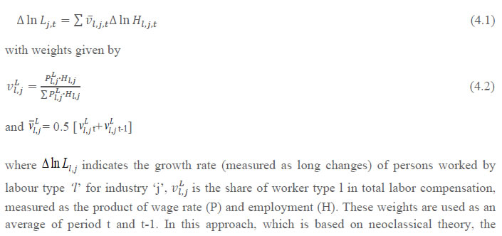 implied assumption is that each worker category is paid their marginal productivities13 and marginal revenues are equal to marginal costs, so the weighting procedure ensures that inputs which have a higher price also have a larger influence in the input index. So, a doubling of number of high-skilled persons worked gets a bigger weight than a doubling of number of low-skilled persons worked. Therefore, the volume growth of labour input as in equation 4.1 can be split into the growth of employment quantity or the number of employed persons and the changes in labour quality index, which is due to the changes in the composition of workers in terms. Let Hj indicate total persons worked in industry ‘j’ by all types ‘l’ in period ‘t’, then 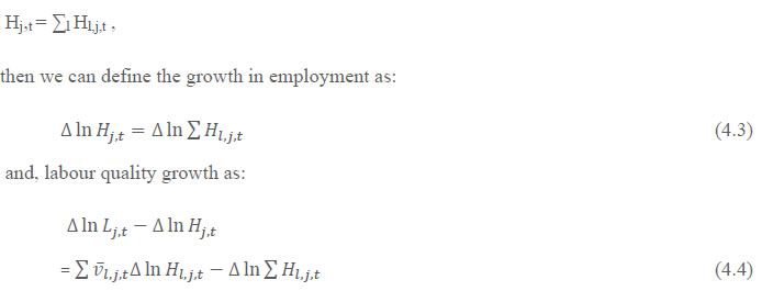 The first term on the right-hand side indicates the change in labour input and the second term indicates the change in total persons employed in sector ‘j’. It can easily be seen that if proportions of each labour type in the labour force change, this will have an impact on the growth of labour input beyond any change in total persons worked. The index of aggregate labour quality thus measures the changes in the composition of labour in the economy. However, the use of this method becomes more and more data intensive as we introduce more classifications of labour such as gender and age groups. Due to data limitation of sample size becoming very small as we try to estimate persons employed and earnings by industry by all the characteristics,14 the present study has computed labour quality index by using only education characteristic in the JGF methodology. Thus, the data required for the labour quality index in the present case, is employment and earnings by education and by industry. The labour quality index15 has been computed using five education categories16 namely- up to primary, primary, middle, secondary & higher secondary, and above higher secondary. There are thus five types of persons employed for each of the 27 study industries. The quality growth rates are estimated for total persons employed in these industries in India for the 38th, 50th, 55th, 61st, 68th and PLFS rounds of NSO. They are then indexed to 1983 (38th round) as the base, so as to assess the temporal changes in labour’s skill and interpolation has been done between the major rounds for values of the intermediate years. Since the series is required from 1980-81, we have extrapolated it backwards from 1983 and the index is recomputed with base 1980-81 equal to 100. Therefore, the following steps have been performed:
The labour input (adjusted labour persons) then can be obtained by multiplying the number of persons employed by the corresponding labour quality index and the labour input growth is finally obtained by combining the growth of persons employed and the growth in the index of labour quality. Appendix C: Definitions of Employment in NSSO employment & unemployment surveys The surveys of NSSO on employment and unemployment (EUS) aim to measure the extent of ‘employment’ and ‘unemployment’ in quantitative terms disaggregated by various household and population characteristics following the three reference periods of (i) one year, (ii) one week, and (iii) each day of the week. Based on these three reference periods three different measures, termed as usual status, current weekly status, and the current daily status, are arrived at. While all these three approaches are used for collection of data on employment and unemployment in the quinquennial surveys, the first two approaches only are used for the purpose in the annual surveys. Usual principal status: In NSS 27th round, the usual principal activity category of the persons was determined by considering the normal working pattern, i.e., the activity pursued by them over a long period in the past and which was likely to continue in the future. For the identification of the usual principal status of an individual based on the major time criterion, in NSS 27th, 32nd, 38th, 43rd rounds, a trichotomous classification of the population was followed, that is, a person was classified into one of the three broad groups ‘employed’, ‘unemployed’ and ‘out of labour force’ based on the major time criterion. From NSS 50th round onwards, the procedure was changed and the prescribed procedure was a two-stage dichotomous one which involved a classification into ‘labour force’ and ‘out labour force’ in the first stage, and thereafter, the labour force into ‘employed’ and ‘unemployed’ in the second stage. Usual subsidiary status: In the usual status approach, besides principal status, information in respect of subsidiary economic status of an individual was collected in all employment and unemployment surveys. For deciding the subsidiary economic status of an individual, no minimum number of days of work during the last 365 days was mentioned prior to NSS 61st round. In NSS 61st round, a minimum of 30 days of work, among other things, during the last 365 days, was considered necessary for classification as usual subsidiary economic activity of an individual. Current weekly status: It is important to note at the beginning that in the EUS of NSSO, a person is considered as worker if he/she has performed any economic activity at least for one hour on any day of the reference week and uses the priority criteria in assigning work activity status. This definition is consistent with the ILO convention and used by most of the countries in the world for their labour force surveys. In NSSO, prior to NSS 50th round and in all the annual surveys till NSS 59th round, data on employment and unemployment in the CWS approach was collected by putting a single-shot question ‘whether worked for at least one hour on any day during the last 7 days preceding the date of survey’. The information so collected was used to determine the CWS of the individuals. This procedure was criticized for being not able to identify the entire workforce, particularly among the women. It was then decided to derive the CWS of a person from the time disposition of the household members for the 7 days preceding the date of survey. The procedure was used for the first time in NSS 50th round. It is seen that the change in the method of determining the current weekly activity had resulted in increasing the WPR in current weekly status approach - more so for the females in both rural and urban areas than for males. The trend observed in NSS 50th round in respect of the WPR according to CWS suggested continuing with the procedure for data collection in CWS in NSS 55th and NSS 61st rounds. Current Daily Status Current Daily Status (CDS) rates are used for studying intensity of work. These are computed on the basis of the information on employment and unemployment recorded for the 14 half days of the reference week. The employment statuses during the seven days are recorded in terms of half or full intensities. An hour or more but less than four hours is taken as half intensity and four hours or more is taken as full intensity. An advantage of this approach was that it was based on more complete information; it embodied the time utilisation, and did not accord priority to labour force over outside the labour force or work over unemployment, except in marginal cases. A disadvantage was that it related to person-days, not persons. Hence it had to be used with some caution.
Chapter 5: Capital Input Series at the Industry Level This chapter outlines the methodology employed to estimate capital input for the 27 industries in the India KLEMS database version 2020. All the productivity calculations in India KLEMS use capital services as the input to production, which is estimated using the approach developed by Jorgenson and Griliches (1967), and outlined in Jorgenson, Gollop, and Fraumeni (1987). The estimation of capital service growth rates is accomplished by first estimating capital stock for different capital assets, and then aggregating across assets after correcting for the differences in their marginal productivities. The main difference between conventional measures of aggregate capital stock and the measures of capital services used in India KLEMS is that the latter accounts for the differences in marginal productivity between different asset types. While the capital stock measures, when accounted for appropriate depreciation profiles, only consider the differences in productivity between different vintages of capital, they do not account for asset heterogeneity. For instance, aggregate capital stock measures would assume that a computer's productivity is the same as that of a car. However, proper measures of capital stock would account for the decline in the efficiency of both computers and cars over their lifetime. Following an overview of the theoretical method to measure capital services (Jorgenson and Griliches,1967;JGF, 1987), the chapter discusses the specific empirical approaches we follow to implement these methods within the constraints of data availability for Indian industries. To measure capital services, using the Jorgenson approach, we need estimates of capital stock for detailed asset types and the shares of each of these assets in total capital remuneration. Using the Törnqvist approximation to the continuous Divisia index under the assumption of instantaneous adjustability of capital, aggregate capital services growth rate is derived as a weighted growth rate of individual capital assets, the weights being the compensation shares of each asset, i.e,    Since our measure of capital input takes account of asset heterogeneity, it was essential to obtain investment data by asset type. We distinguish between 3 different asset types – construction, transport equipment, and machinery (includes ICT and non-ICT machinery).21 We exploit multiple sources of information for the construction of our database on capital services. This includes the National Accounts Statistics (NAS) that provide information on broad sectors of the economy, the Annual Survey of Industries (ASI) covering the organized manufacturing sector, the National Sample Survey Office (NSSO) rounds for unorganized manufacturing and Input-Output tables. Even though we use multiple sources of data, our final estimates are fully consistent with the aggregate data obtained from the NAS. In addition, our approach to capital measurement is consistent with international practices such as the EU KLEMS22, which ensures the possibility of international comparisons. In what follows, we discuss the various sources of data for asset wise investment and the construction of the relevant variables, in detail.  (a) Asset-wise investment for broad sectors of the economy Industry-level estimates of capital input require detailed asset-by-industry investment matrices. NAS provides information on aggregate capital formation by industry of use for nine broad sectors, which, nevertheless, was not sufficient for our purpose. Therefore, we have collected more detailed data on assets and industries from the CSO.23 This is the data underlying the published aggregate gross fixed capital formation by the broad industry groups, separately for public and private sectors. For those sectors for which the investment matrices were not available from CSO, we gather information from other sources (e.g. ASI for organized manufacturing and NSSO surveys for unorganized manufacturing) and benchmark it to the aggregate investment series from the National Accounts. The data used in the current version of the India KLEMS is based on the revised NAS with 2011-2012 base, and is available only since 2012. Therefore, for earlier years, we extrapolate the series using growth rates from previous version of the data. However, there were slight differences between the industry groups available in the current release of the NAS data and the previous ones (see Table 5.1), which required some matching of sectors before combining the two series. Table 5.2 provides an overview of asset types available in NAS and their corresponding asset types used in our study. Investment in education and health are obtained directly from national accounts for the period after 2012, for each asset. For years before 2012, we assume the trend in the distribution of output, in order to split the total investment in the aggregates of these sectors into sub-sectors.
Total investment in each asset category is calculated as the sum of private and public sector investment in each asset. Investment in transport equipment is not available separately for private sector. We tried several approaches to impute the private sector transport equipment data. The first was to use the share of transport equipment in non-departmental enterprises. More specifically, we apply the non-departmental enterprise transport equipment to machinery & equipment (including transport equipment) ratio to machinery & equipment in private sector for each industry to obtain industry wise transport equipment for private sector. We take non-departmental enterprise only, rather than the entire public sector, as it may be more realistic as it consists of public sector companies and statutory corporations, excluding administrative sector. However, the sum of industry estimates generated by this approach was not consistent with the reported aggregate private sector transport equipment. Therefore, we take a second step here, which is to use the industry distribution from this series and apply it to the published total private sector transport equipment data. The estimated transport equipment is then subtracted from each industry’s total machinery & transport equipment data, to obtain machinery in private sector as a residual. However, this approach generates many negative numbers in transport equipment in private sector, particularly in transport services. Therefore, we follow a third approach, which is what we finally use in the database. We first distribute the NAS total machinery in the private sector using the industry distribution of machinery and transport equipment. These estimates are then subtracted from each industry’s total machinery & transport equipment data to obtain the transport equipment investment in the private sector industries. Using this approach, we could generate investment in transport equipment by industries for the period 1950-2016. However, since 20216-2017, as we did not obtain detailed asset/industry-wise data on capital formation from the CSO, we relied solely on publicly available data from the National Accounts. The publicly available data contains more detailed information now, compared to what it used to be in the past. Therefore, the reliance on the NAS public data did not create too many challenges. However, there were two outstanding issues. The first was regarding the imputation of transport equipment. Data on transport equipment was not separately available in this data. Therefore, we assumed the share of transport equipment in the total machinery and equipment group in 2016-2017 to remain constant to create nominal investment in transport equipment in the subsequent years. The nominal investment was deflated using GFCF deflator for transport equipment (see section (c)). The second issue was related to the split of the manufacturing sector into registered and unregistered manufacturing. Since NAS provides the investment data for the aggregate manufacturing sector, we use information from the Annual Survey of Industries (ASI) and NSSO unorganized surveys to distribute the aggregate GFCF across industries (see section b). However, NAS does not provide the split between registered and unregistered manufacturing since 2016, making it challenging to use ASI and NSSO data to split the aggregate manufacturing. Nevertheless, NAS provides a division between the corporate sector, public sector, and household sector. As a quick fix, in the current version of the data, we consider the household sector as a proxy for unregistered and the corporate and public sector as a proxy for the registered sector. As mentioned earlier, the updates for years since 2017-2018 are solely based on published aggregate GFCF data from the National Accounts. In the 2019 version of the India KLEMS, we considered the 2012-2016 detailed asset-wise data by industries provided by the CSO as such and extended the data for 2017-2018 using the published aggregates. However, in the 2020 version of the data, we changed this approach, as there were some discrepancies between the published NAS totals and the detailed asset-industry data. While extending the past series of detailed asset-wise investments forward for years since 2017-2018 using the NAS-published headline series, we now consider the published NAS series as the benchmark since 2012. Then we apply the industry distribution of the 2012-2016 detailed series obtained previously from the CSO. The current approach is more appropriate and ensures a complete consistency with the NAS-published series. However, it may cause some changes in the capital service growth rates compared to the last release. As discussed at the beginning of this section, as we use multiple vintages of GFCF data from various revisions of national accounts, we extrapolate the 2011-2012 base nominal GFCF series backwards using growth rates from the 2004-2005 series. Using. While doing this, in the previous versions of the KLEMS data, we first extrapolated each individual industry in the NAS detailed data and then aggregated them to the KLEMS sector. For instance, suppose we have n NAS industries (i=1,...,n) that constitute a KLEMS sector j (e.g., the KLEMS sector transport & storage consists of NAS sectors railways, air transport, water transport, road transport, other public transport, other private transport, other transport services, and storage). In the previous versions of the data, we extrapolated the nominal GFCF in the 2012 series for each of these n sectors individually backward using the growth rates from the nominal GFCF series from the 2004 version. We change this approach in the current 2020 version to extrapolate after aggregating detailed data to the KLEMS sector, as we observe significant inconsistencies in the detailed industry data for some industries between the two versions of the NAS. Therefore, we first aggregate the nominal GFCF for the KLEMS sector and then extrapolate it backward for each KLEMS industry. More formally, the approach we followed in KLEMS version 2019 was: 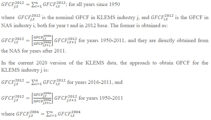 The change in the aggregation procedure causes some differences in the historic GFCF growth rate for the KLEMS sector j for the period 1950-2011. This difference in the GFCF growth also leads to a historical revision of capital stock growth rates for the entire series in some industries (e.g., agriculture, which is the sum of crops, fisheries, forestry; utility sector, which is the sum of electricity, gas, and water supply; transport services, which is the sum of different transport services, storage, etc.), as capital stock is a cumulative sum of investment stream over the years. While it may be accurate to use detailed industry data to extrapolate backward (the earlier approach), the magnitude of the fluctuation might affect the quality of the data. Moreover, the current approach is consistent with the approach taken for gross value added in the KLEMS database. (b) Asset-wise investment for non-NAS sectors NAS provides data only for 9 broad sectors, while we have 27 industries, which necessitated further splitting of some of the NAS sectors. This includes aggregate manufacturing (registered and unregistered separately for the period 1950-2016) with 13 sub sectors; other services into 4 sub sectors; and real estate activities and business services into 2 sub sectors. The manufacturing sector investment data was disaggregated into 13 subsectors at the 2-digit level of NIC 1998 using ASI and NSSO data, which will be discussed in detail subsequently. Investment series in service sector has been split into sub sectors using two alternative approaches–value added shares, and capital/labour ratio in the higher aggregate industry. However, the final data used are based on value added shares, as a sensitivity analysis did not show a significant difference between the two. Registered (organized) Manufacturing: In order to split the aggregate capital formation in organized manufacturing sector into 13 study sectors, we use the ASI. However, the published data does not provide any asset wise investment information; it consists of only the aggregate capital formation or the book value of fixed capital. Most studies in the past have measured gross investment as the difference between book value of asset in period t and in period t-1 and add depreciation in period t to that. This approach has the deficiency of comparing two different samples reported in two different years, where the number of firms/factories might be different. In particular, while using this approach at industry level, for detailed asset categories, it might generate massive negative investment. We follow an alternative approach, following ASI’s definition of gross fixed capital formation (GFCF). ASI defines GFCF as actual additions (newly purchased, second hand and own construction) minus deductions plus depreciation adjustment for discarded assets during the year. This approach is based on a single year’s sample and helps to avoid potential huge negative investment series, and is also consistent with published ASI GFCF series. The yearly detailed volumes beginning 1964-65 were used to derive the gross fixed capital formation by asset type directly. For the years 1964-1978, the relevant data are obtained from published detailed volumes. For the period, 1983-84 to 2004-05 ASI has generated detailed tables from Block C of ASI schedule that contain data on fixed assets. Data for missing years are interpolated using the changes in investment using book value method. Table 5.3 provides an overview of the asset categories available in ASI, and the relevant asset categories in our study to which they are attributed. Though ASI provides investment in land, for reasons of NAS consistency we exclude it from our database. Once investment in each of these assets and industries are generated using ASI data, we apply this industry-asset distribution to the published aggregate NAS GFCF series for organized manufacturing sector. It may also be noted that from 1960-61 to 1971-72, ASI data are for the census sector and from 1973-74 onwards they are for the factory sector. In order to make these two series comparable over years, we convert the data prior to 1972 to factory sector using the factory/census ratio in 1973. Thus, after these adjustments, we obtain investment data for 13 manufacturing sectors, by asset types, consistent with the NAS aggregate for registered manufacturing. This approach was accurate for the period 1950-2016 when the NAS provided aggregate registered manufacturing GFCF data. For the years after 2016, since when NAS does not provide registered manufacturing aggregate, we proxy registered manufacturing by the sum of public sector and corporate sector. Unregistered (unorganized) Manufacturing: The data required for creating the gross investment series for the 13 sectors of the unorganized manufacturing sector are obtained from various rounds of NSSO surveys on unorganized manufacturing. We use 6 rounds of NSSO surveys that cover the period 1989-2016. These are 45th round (1989-90), 51st round (1994-94), 56th round (2000-01), 62nd round (2005-06), 67th round (2010-11) and 73rd round (2015-16). Unit level data has been aggregated to 13 industries using the appropriate concordance tables. NSSO provides net addition to owned assets during the reference year within the block of fixed assets, and we use this as a measure of our investment. Asset classification in NSSO has changed over various rounds, and therefore, we have tried to match these with our classification as shown in Table 5.4. The investment series arrived at for six rounds were interpolated to obtain the annual time series of unorganized gross fixed capital formation by asset type. As in the case of registered sector, once the investment by asset types across industries are constructed, the asset-industry distribution is applied to the published NAS aggregate GFCF in unregistered manufacturing to obtain NAS consistent GFCF by asset type and industries. (c) Investment Prices by Asset Types In order to compute asset wise capital stock using PIM (equation 5.3) and rental price (equation 5.4), we require asset wise investment price deflators. Since CSO has provided us with investment data by industries and assets both in current and constant prices, we could derive the price deflators with base 2011-2012. For years before 2011, prices were spliced using 2004-2005 base investment deflators. These deflators are directly used for all the three asset categories we have. Since there was no separate asset wise data available for transport equipment in 2017-2018, the investment deflator for transport equipment from 2016-2017 was extrapolated using the trend in the investment price of total machinery & equipment, obtained from NAS. (d) Initial Stock, Depreciation Rates and Rate of Return As is evident from equations 5.1 to 5.4, our estimates of capital input require time-series data on asset wise capital stock. Capital stock has been constructed using perpetual inventory method (PIM), where the capital stock (S) is defined as a weighted sum of past investments with weights given by the relative efficiencies of capital goods at different ages, which requires data on current investment by asset types, investment prices by asset types and depreciation rate. Also, for the practical implementation of PIM to estimate asset wise capital stock, we require an estimate of initial benchmark stock (see Erumban, 2008b for an in-depth discussion on this issue). NAS provides estimates of net capital stock since 1950 for all the broad sectors in its Statement 17: Net Fixed Capital Stock by industry of use. We take the NAS estimate of real net capital stock in 1950 (in 1999-2000 prices) as our benchmark stock for all non-manufacturing sectors, and for manufacturing sectors the same is taken for the year 1964.25 However, since the NAS estimate is available only for broad sectors and for aggregate capital, we use our industry-asset distribution of GFCF in order to create net fixed capital stock estimates by asset type for all the 27 sectors. The approach to split asset-wise capital stock is changed in the 2020 version of the India KLEMS database. Instead of using the GFCF distribution, we use the distribution of net capital stock by assets, available from the detailed asset data obtained from the CSO. Since the initial stock depreciates over the years, the impact of this change in distribution on the capital stock will vanish over the years at the individual asset level. However, as it changes the distribution of assets in the total capital stock, these compositional changes tend to have a visible impact on the aggregate capital stock, causing a historical revision of capital stock growth rates in some industries (esp. transport and storage, education, hotels and restaurants, electricity, transport equipment, etc.). NAS also provides detailed tables on assumed life of assets used for computing capital stock, for private units, administrative units as well as departmental and non-departmental units by asset types.26 We use these estimates of lifetime to derive appropriate depreciation rates for non-ICT assets, using a double declining balance rate. Following the NAS, we assume 80 years of lifetime for buildings, 20 years for transport equipment, and 25 years for machinery and equipment (see Appendix 26.2; CSO, 2007). The final depreciation rates used in the study are given in Table 5.5 by asset type. Subsequently, we build our capital stock series by asset types for all the 27 industries using our GFCF series from 1950 (1964) onwards for the non-manufacturing (manufacturing) sectors. Our measure of capital input is arrived using equation (5.1), for which we also require estimates of rental prices (see equation 5.4). Assuming that the flow of capital services is proportional to the capital stock at individual asset level, aggregate capital flows can be obtained using a translog quantity index by weighting growth in the stock of each asset by the average shares of each asset in the value of capital compensation, as in (5.1). The rate of return (i) in equation (5.4) represents the opportunity cost of capital, and can be measured either as internal (or ex post) rate of return, or as an external (ex ante) rate of return.27 This issue will be addressed in the further revisions of the data. The present version of the database uses an external rate of return, proxied by average of return on government securities and prime lending rate obtained from the Reserve Bank of India28. Therefore, we use a real rate, which is net of capital gain. Hence, the capital gain component in equation (5.4) is excluded while estimating rental price using external rate of return, obtaining  Where r is the real rate of return, nominal interest rate adjusted for consumer price inflation rate. The consumer price indices (CPI) are obtained from IMF and World Bank. 5.3 Outstanding issues The measures of capital input available in India KLEMS are based on only three asset categories, construction, machinery, and transport equipment. Therefore, it does not consider the enormous and distinct role of ICT capital in contributing to productivity and growth. The absence of ICT estimates in the database is driven by insufficient data on investment in ICT assets, such as hardware, software, and communication equipment in the National Accounts. However, during recent years, NAS has extended its asset coverage to include software and ICT equipment. Erumban and Das (2016) have made some estimates for the aggregate economy using input-output tables for ICT equipment and relying on NAS for software investment. Similarly, Erumban and Das (2020) have made some initial estimates of ICT capital by industries, which still remains a challenging task. Nevertheless, now that more data is available from NAS, it is possible to explore this further, and future extensions of the database may explore this. Similarly, following the SNA 2008 guidelines, the NAS now provides estimates of intangible capital such as intellectual property and research and development (R&D), which may be a useful extension to the capital input database. Two additional challenges are arising since the new system of national accounts. The first is the lack of separate data on registered and unregistered manufacturing, which poses challenges in using ASI and NSSO data to split aggregate manufacturing data into 13 industry groups. Instead of the registered and unregistered split, CSO now provides a division between the household and corporate sectors. We currently address this challenge by considering the household sector as unregistered manufacturing and the sum of public and corporate sectors as a registered sector. The second challenge is the lack of separate data on transport equipment and machinery assets in the new series of national accounts, which follows United Nation's System of National Accounts (SNA)-2008. Although, for the time being, we adopt ad-hoc approaches to fix this, it cannot be adopted on a long-term basis, which might necessitate combining transport equipment and machinery to one single asset. Finally, as mentioned earlier, the debate on whether it is appropriate to use an external rate of return or an internal rate of return is unsettled in the literature. It may be worth exploring estimates of capital using the internal rate of return. Chapter 6: Intermediate Input Series at the Industry Level In this section, we describe the basic approach we have used to derive the volume series of Intermediate Inputs namely –Energy input (E), Material input (M) and Services input (S). This breakdown of intermediate inputs can be used for extending the growth accounting exercises, but also convey interesting information about changing pattern in intermediate consumption (see e.g., JHS 2005, chapter 4) The methodology for measuring industry output, intermediate inputs and value added was developed by Jorgenson, Gallop and Fraumeni (1987) and extended by Jorgenson (1990 a). The cornerstone of this approach is a time series of input output (IO) tables which gives the flows of all commodities in the economy, as well as payments to primary factors. Every commodity is accounted for, whether produced by a domestic source or imported, and every use is noted, whether purchased by an industry or by a final demand element. All payments to factors of production i.e., labour and capital is accounted for so that all income elements of GDP are included. The methodology of constructing time series on energy, material and services inputs for the European economy has been elucidated in Timmer et al. (2010, Chapter 3). Following a similar approach as explained in Jorgenson et al. (2005, Chapter 4) and Timmer et al. (2010, Chapter 3), the time series on intermediate inputs for the India KLEMS project have been constructed. Definition of EMS: As in EU KLEMS, this study identifies three main categories of Intermediate inputs. They are classified as follows:
Intermediate Inputs are broken down into energy, material and services, based on input output transaction tables using a standard NIC product classification. The following five energy types (and products) have been classified as the Energy input:
The following fourteen input items have been classified as the Service input:
All other intermediate inputs barring the above mentioned nineteen inputs are classified as material input. The key building block for constructing time series on Intermediate Inputs at current prices, as explained in Jorgenson et al. (2005, Chapter 4), is the input-output transaction tables, that is, the inter industry transaction tables that provide a description of which industries produce each product and which industries use them. The input-output table gives the inter-industry transactions in value terms at factor cost presented in the form of commodity x industry matrix where the columns represent the industries and the rows as group of commodities, which are the principal products of the corresponding industries. Each row of the matrix shows in the relevant columns, the deliveries of the total output of the commodities to the different industries for intermediate consumption and final use. The entries read down industry columns give the commodity inputs of raw-materials and services, which are used to produce outputs of particular industries. The column entries at the bottom of the table give net indirect taxes (NIT) (indirect taxes – subsidies) on the inputs and the primary inputs (income from use of labour and capital), i.e., Gross Value Added (GVA). As the IOTT is in the form of commodity x industry matrix, the row totals do not tally with the column totals. The difference between each column and the corresponding row totals is due to the inclusion of the secondary products, which appear particularly in the case of manufacturing industries. This is so because by-products are also manufactured by industries in addition to their main products. Thus, while determining the entries in the rows, a by-product of an industry is transferred to the sector (commodity row), whose principal product is the same as the by-product under reference. The columns, however, show the total of principal products and by-products of each industry. All the entries in the IOTT are at factor cost, i.e., excluding trade and transport charges and NIT. The Input Flow Matrix at factor cost, published by CSO, for 1978 is a 60 x 60 matrix. The absorption matrices for 1983, 1989, 1993 and 1998 have 115 sectors. However, a detailed 130 sector absorption (commodity x industry) matrix for the Indian economy has been published from 2003-04 onwards. The scheme of sector classification adopted in IOTT 2015-1629, IOTT 2007-08 and IOTT 2003-04 vis-à-vis, IOTT 1983-84, IOTT 1989-90, IOTT 1993-94 and 1998-99 has undergone significant change with the disaggregation of some of the sectors, which have become significant in early 2000s.
The methodology for computation of Intermediate Input Series for 27 Industries from 1980-2018 at current and constant prices is explained in steps. Step 1: Concordance is done between IOTT and study industries
Step 2: Obtaining estimates for Material, Energy and Service Inputs for 27 Industries, in benchmark years
Thus, for each of the benchmark year, estimates are obtained for Material, Energy and Service Inputs that has been used to produce Gross output in the 27 different India KLEMS Industries. Step 3: Projecting a time series (1980 to 2018) of proportions of Material, Energy and Service Inputs in Total Intermediate Inputs for each of the 27 industries
There exists some abnormal fluctuation in the proportions of Material Inputs, Energy Inputs, and Service Inputs in Total Intermediate Inputs for benchmark years. In that case, we drop that specific benchmark proportion and linearly interpolate of the adjacent benchmark proportions to estimate proportion for intervening years. For the industry ‘Wood & Wood Products’, we estimated proportions of Material Inputs, Energy Inputs, and Service Inputs in Total Intermediate Inputs from SUT 2015-16 instead of Input Output Transaction Table 2015-16. This has been done because the relevant proportions in SUT 2015-16 is believed to be making a more correct assessment. For the industry group ‘Coke, Refined Petroleum and Nuclear Fuel’, we estimated proportions of Material Inputs, Energy Inputs, and Service Inputs in Total Intermediate Inputs from ASI data instead of Input Output Transaction Table. This has been done because the relevant proportions differed significantly between the input-out tables and ASI, and the latter is believed to be making a more correct assessment of energy inputs used in the Coke and Petroleum products industry. For example, coal consumed in the Coke industry is taken primarily as material rather than energy. From IOTT it is difficult to estimate how much of coal consumption is for energy purposes and how much as material input, where ASI provides details information about energy consumption by energy inputs like: coal, electricity, petroleum and others including natural gas. Step 4: Consistency with NAS The projection of intermediate input vector, using IOTT in Step 3 needs to be consistent with the estimated output from NAS.
1. For Benchmark years: Ratio of Total Intermediate inputs from NAS to that from IOTT is adjusted proportionately to the absolute value of Energy Inputs/Material Inputs/Service Inputs obtained from IOTT. 2. For Intervening Years: The interpolated proportions of Energy Inputs, Material Inputs and Services Inputs obtained from IOTT, is applied directly to the total intermediate inputs from NAS to get each inputs share. Two examples have been given below for the Construction sector: In the examples above, we can see that the total value of intermediate input exactly matches the gap between Gross output and Value added. Similar adjustments have been made to construct the input series for all the other 27 study industries from 1980-2018. For every benchmark year where IOTT is available adjustment ‘A’ has been done. For every non-benchmark year, where IOTT is not available and an intermediate input vector has been projected, adjustment ‘B’ has been done to generate the comprehensive time series of Intermediate inputs consistent with the official National Accounts. Steps 1-4: This gives a time series of Material, Energy, and Service Inputs for 27 study Industries from 1980 to 2018 at current prices. Steps 5 and 6 below, explain the methodology for computation of Intermediate Input Series for 27 study Industries from 1980-2018 at constant price. The approach followed here is to first form the aggregates of materials, energy and services at current price for each study industry from the benchmark Input Output tables and then develop deflators of Materials, Energy and Service Inputs for each of the 27 study Industries separately. Step 5: Constructing Deflators of Materials, Energy and Service Inputs for 27 study Industries separately
Step 6: Computing Time Series on Intermediate Input for 27 study Industries from 1980-2018, Constant prices
Thus, we have a time series of Material, Energy and Service Inputs for 27 study Industries at constant prices. Firstly, input output transaction tables are generally available on a five-year interval period and this necessitates interpolation and assumption of constant shares in some cases, to construct the entire time series of EMS from 1980 to 2018. Secondly, unlike studies using detailed survey data, we have to assume that all buyers pay the same price for each commodity because there is no information about price divergences. Thirdly, the estimated time series of Intermediate Inputs at constant price will not be consistent with the intermediate input of NAS at constant price i.e., the deflated value of intermediate input cannot match the gap between value added and gross output at constant price from NAS. This is because; NAS uses a single deflation method to estimate Gross Value Added and Gross Output at constant price. Chapter 7: Factor Income Share Series at the Industry Level The distribution of income between capital, labour and intermediate inputs, is an important element in growth accounting because income shares, under conditions of competitive markets, can be used to measure the contributions each factor makes towards output growth. 7.1 Methodology for Measuring Labour Income Share Series Under the assumption of constant returns to scale with two factors of production i.e., labour and capital, the sum of the labour income share and capital income share is 1. The labour income share is defined as the ratio of labour income to GVA. Capital income share is accordingly obtained as one minus labour income share. There are no published data on factor income shares in Indian economy at a detailed disaggregate level. National Accounts Statistics (NAS) of the CSO publishes the NDP series comprising of compensation of employees (CE), operating surplus (OS) and mixed income (MI) for the NAS industries. The income of the self-employed persons, i.e., mixed income (MI) is not separated into the labour component and capital component of the income. Therefore, to compute the labour income share out of value added, one has to take the sum of the compensation of employees and that part of the mixed income which are wages for labour. The computation of labour income share for the 27 study industries involves two steps. First, estimates of CE, OS and MI have to be obtained for each of the 27 study industries from the NAS data which are available only for the NAS sectors (see Table 7.1). Second, the estimate of mixed income has to be split into labour income and capital income for each industry for each year (except for those industries for which the reported mixed income is zero, for instance, public administration). Basis data sources used for the computation of labour income share are NAS, ASI and unit level data of survey of unorganized manufacturing enterprises. These data sources are used to obtain estimates of CE, OS and MI for each of the 27 study industries. For splitting the labour and non-labour components out of the mixed income of self-employed, the unit level data of NSS employment-unemployment survey are used along with the estimates of CE, OS and MI basically obtained from the NAS. a) Construction of Labour Income Share Series in Gross Value Added The estimation of labour income share for the 27 study industries has been done in two steps, as discussed below. Step 1: Estimation of CE, OS and MI for the 27 study Industries NAS provides estimates of compensation of employees (CE), operating surplus (OS) and mixed income (MI) for the 9 NAS industries in different annual Sequence of National Accounts reports. In the Back Series with base 2011-12, NAS updated the estimates of GVA for the years prior to 2011-12, but did not provides the updated estimates of CE, OS and MI. Therefore, for 1980-81 to 2011-12 period, we proportionally adjusted the CE, OS and MI series corresponding to the updated GVA estimates. For some industries under study, for instance (i) Agriculture, forestry & logging and fishing, (ii) Mining & Quarrying, (iii) Electricity, gas and water supply and (iv) Construction, the required data are readily available from NAS. For others, the estimates available in NAS have to be distributed across the study industries. In certain cases, the estimates of CE, OS and MI for a particular NAS sector have been distributed across constituent study industries proportionately in accordance with the gross value added in those industries. Estimate of factor incomes for ‘other services’ in NAS, for instance, has been split into estimates for (i) Education, (ii) Health and Social Work, and (iii) Other Community, Social and Personal Services including Renting of Machinery and Business Services, and Private Household with Employed Persons. Before 2011-12, NAS provides estimates of factor incomes for registered manufacturing and unregistered manufacturing, but not for individual manufacturing industries. However, 2011-12 onwards NAS disaggregated the manufacturing sector in corporate sector and household sector. The NAS estimates of factor incomes for registered manufacturing and corporate sector have to be split into various manufacturing industries considered in the study (13 in number) using ASI data. The reported CE in NAS for registered manufacturing and corporate sector has been distributed into those 13 industries in proportion to the reported ASI data on emoluments for various industries. In a similar way, using ASI data, the estimate of OS for registered manufacturing and corporate sector has been distributed. Emoluments are subtracted from gross value added for various industries yielding capital income. The share of different industries in aggregate capital income of organized manufacturing indicated by the ASI data is used to split the estimate of OS for registered manufacturing and corporate sector reported in the NAS. The methodology applied for unregistered manufacturing and household sector is similar. The published results and unit level data of survey of unorganized manufacturing industries have been used for this purpose. The estimates of wage payments (to hired workers) in different industries have been used to split (proportionately) the estimate of CE in the NAS for aggregate unregistered manufacturing. The estimated wage payment is subtracted from the estimated value added to obtain an estimate of capital income and mixed income of the self-employed in various unorganized manufacturing industries. The estimate of MI provided in NAS for unregistered manufacturing and household sector has then been proportionately distributed across industries using the estimate of capital income and mixed income of the self-employed in various industries that could be formed on the basis of published results and unit level data of survey of unorganized manufacturing industries. Unlike the ASI data for organized manufacturing, the data for unorganized manufacturing enterprises are available for only select years. The proportions mentioned above could therefore be computed only for those select years (data for six rounds have been used; these are for 45th Round (1989-90), 51st Round (1994-95), 56th Round (2000-01), 62nd Round (2005-06), 67th round (2010-11) and 73rd Round (2015-16)). It has accordingly, been necessary to resort to interpolation/ extrapolation to obtain the relevant proportions for other years. Step 2: Splitting of MI into Labour Income and Capital Income As explained above, the income share of labour is computed as: 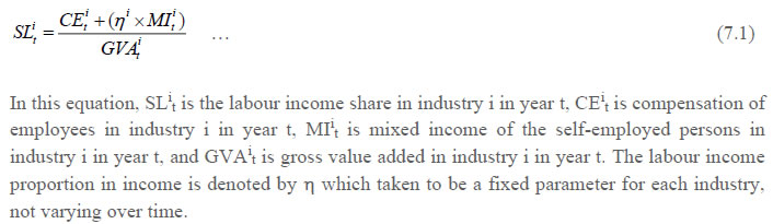 The derivation of the GVA series for different industries has been briefly explained in Chapter 2. The derivation of CE and MI series has been explained in step I above. Therefore, only the estimation method of ƞ needs to be described. The estimation of ƞ has been done with the help of NSS survey-based estimates of employment of different categories of workers (number of persons and days of work) and wage rates (which has been described briefly in chapter 4) coupled with estimates of MI, basically obtained from the NAS. Two approaches have been taken to get an estimate of ƞ, and the labour income share series for different industries finally adopted in the study makes use of an average of the estimates of ƞobtained by the two approaches. In the first approach, an estimate of labour income of self-employed workers has been made for each study industry for eight years, 1983-84, 1987-88, 1993-94, 1999-00, 2004-05, 2009-10, 2011-12 and 2015-16 on the basis of the estimated number of self-employed, wage rate of self-employed and the number of days of work per week. The industry-wise estimates of number of self-employed, wage rate of self-employed and the number of days of work per week have been made from unit records of NSS employment-unemployment survey (major rounds) of 1983, 1993-94, 1999-00, 2004-05, 2011-12, and PLFS of 2017-18 and 2018-19. The estimates of the number of self-employed, wage rate of self-employed and the number of days of work per week provide an estimate of the annul labour income of self-employed workers which is divided by the mixed income of self-employed (derived from NAS) to get an estimate of ƞ. For five industries, the ratio in question has been computed and applied. For the other 22 industries, the ratio in question has been computed after clubbing the industries into 11 industry groups.30 In the latter case, a common ratio computed for group of industries has then been applied to constituent industries. The list of industries or industry groups for which ƞ has been estimated is given in table 7.2. In the second approach, the NSS data are used to compute the following ratio: the ratio of labour income of self-employed workers to the labour income of regular and casual workers. Let this be denoted by θ. Then, the estimate of CE provided in the NAS is multiplied by θ to obtain an estimate of the labour income component out of the MI reported in the NAS. The labour component of MI divided by total MI gives an estimate of ƞ. In case the estimated labour component of MI exceeds the estimate of MI, the estimate of ƞ has been taken as unity. Examining the estimates obtained by the first approach, it was found that the estimated labour income share out of mixed income varied significantly among the estimates for the seven years for which the ratio in question has been estimated. The estimates of ƞ obtained by the second approach has the problem that in a number of cases, the estimated labour component of MI exceeds the estimate of MI given in the NAS, and therefore ƞ is taken as one. The method finally adopted is as follows: (a) The average value of ƞ has been computed for each industry or industry group by taking the estimates for the years 1983-84, 1987-88, 1993-94, 1999-00, 2004-05, 2009-10, 2011-12 and 2015-16. This has been done separately for the estimates based on approach-1 and those based on approach-2. (b) The estimates of ƞ obtained for each industry or industry group by the two approaches have then been averaged. (c) Having obtained an estimate of ƞ, equation 6.1 given above has been applied to compute the labour income share. b) Construction of Factor Income Share Series in Gross output The income share of labour, capital and intermediate inputs in Gross output has been computed using the following steps:
The splitting of unorganized sector factor incomes into individual industries has been done using unorganized survey results. The proportions computed for 1983-84 has been applied for the period 1980-81 to 1983-84. While there were surveys of unorganized manufacturing enterprises in 1978-79 the survey results have not been used for estimation of factor incomes in different industries of the unorganized manufacturing sector. Chapter 8: Growth Accounting Methodology This chapter deals with the methodology of measurement of total factor productivity (TFP) growth for individual industries in the KLEMS framework and the aggregation from industry level productivity measures to measures for broad sectors and the economy as a whole. The methodology of analysis of sources of gross output growth at the individual industry level and sources of GVA (Gross Value Added) or GDP growth at the broad sector level and economy level will also be presented in this chapter 8.1 Methodology for Measuring Productivity Growth at the Industry level The production function Our measurement of TFP growth for different industries of the Indian economy is based on a gross output production function for each industry j:  Y is industry gross output, L is labour input, K is capital input and E, M and S are intermediate inputs-namely energy, material and services and T is an indicator of technology for industry j. All variables are indexed by time (t subscript is suppressed). There are several things to note about the production function - (1) all variables are aggregates of many components that have been discussed in the earlier report/chapters; (2) we assume that the industry production function is separable in these aggregates; (3) time (indicator of technology) enters the production function symmetrically and directly with inputs. An important feature of the gross output approach is the explicit role of intermediate inputs. In our study, we have considered three intermediate inputs - energy, material and services and this is important as we may find that intermediate inputs are the primary component of some industries outputs.31 Failure to quantify intermediate inputs leads us to miss both the role of key industries that produce intermediate inputs and the importance of intermediate inputs for the industries that use them. In order to estimate the production function at constant prices, the industry level price data is used for output, capital, labour and intermediate inputs, e.g., PYj; PLj, PKj; PEj. PMj, PSj. We assume that all industries face the same input price. The industry price of an input varies across industries due to compositional effects as industries expend different shares of their investment on each type of asset. The same is true for all inputs. Total Factor Productivity To estimate TFP growth, we begin with the fundamental accounting identity for each industry where the value of output equals the value of inputs.  Under specific assumptions of constant returns to scale and competitive markets, we can define TFP growth as  Rearranging equation (8.3), yields the standard growth accounting decomposition of output growth into the contribution of each input and the TFP residual  where the contribution of an input is defined as the product of the input’s growth rate and its two period average value share. We can further decompose the contribution of each input into a quantity and quality component. As discussed earlier, the quality component represents substitution between H components, while the quantity component represents the increases in each detailed input. Our extended decomposition of the sources of output growth is given as follows  Where Z is the stock of industry capital, Qk is the capital quality, H is number of persons employed and Ql is the quality of labour. 8.2 Methodology for Aggregation across Industries In the analysis presented in the above section, gross value of output (GVO) is taken as the measure of output of an industry and TFP growth was estimated using the gross output function framework in which capital, labour, materials, energy and services are taken as five inputs. The Törnqvist index is applied to estimate TFP growth for each year during 1980-81 to 2018-19, which yielded an index of TFP for each industry for that period, permitting estimation of trend growth rate in TFP for the period under study (1980-81 to 2018-19). The method of estimation of TFP growth for individual industries described in section 8.1 cannot be readily applied to a higher level of aggregation. The main problem is that gross value of output cannot be added across industries to generate a measure of output at a higher level of aggregation, say for the economy or of any of the broad sectors. It becomes necessary therefore to consider appropriate methods of aggregation across industries consistent with the gross output function specification of technology at the individual industry level. It is needless to say that one has to use the concept of value added to define an appropriate measure of output at the economy or broad sector level, but even here there are important issues of aggregation, i.e., how value added in different industries should be combined. A very useful discussion of the issues involved is found in Jorgenson et al. (2005). There are three approaches to estimating TFP growth at an aggregate level. This is discussed in detail in Jorgenson et al. (2005). The first approach is called aggregate production function approach. This approach assumes the existence of an aggregate production function (say, at the level of the economy or at the level of manufacturing or services sector). An essential condition is that the production function be separable in primary inputs. Let the production function for a particular industry be defined as:  where Y denotes gross output, X intermediate input (in turn a combination of materials, energy and services), K capital input, L labour input and T time (representing technology). Then, the concept of value added requires the existence of a value-added function which in turn requires that the above production function be separable in K, L and T, i.e., the production function should take the following form:  In this equation, V (.) is the value-added function. V denotes value added. Besides the condition of separability of the production function described above, a number of highly restrictive assumptions have to be made for the aggregate production function approach. These include: (a) the value-added function is the same across all industries up to a scalar multiple, (b) the functions that aggregate heterogeneous types of labour and capital must be identical in all industries, and (c) each specific type of capital and labour receives the same price in all industries. With these assumptions made, real value added at the aggregate level becomes a simple addition of real value added in individual industries. In notation,  where Vi is value added in the ith industry and V is the aggregate value added. Given aggregate value added and somewhat similarly defined aggregate capital and labour input, TFP growth at the aggregate level can be computed. The second approach to aggregation is the aggregate production possibility frontier approach. It also needs the separability condition described in equations 8.8 and 8.9 above, as in the case of the aggregate production function approach. The main difference between the aggregate production function approach and the aggregate production possibility frontier approach is that the latter relaxes the assumption that all industries must face the same value added function. Thus, the price of value added is no longer assumed to be the same across industries. The implication is that the aggregate value added from the aggregate production possibility frontier is given by the Törnqvist index of the industry value added as:  In this equation, wi is the share of industry i in aggregate value added in nominal terms. Thus, defining PV,i as the price of value added in industry i and Vi as the real value added in industry i, the share in question may be defined as:  and the two-period average is defined as:  Since each industry is subject to a production function separable in capital, labour and technology, as defined in equation 8.9, real gross output, real value of intermediate inputs and real value added of industry i in a particular year t should satisfy the following relationship:  In this equation, uV and uX are the shares of value added and intermediate inputs in the gross value of output in nominal terms. Given data on growth in gross output and growth in intermediate input of a particular industry, the above equation yields the growth in real value added of that industry. TFP growth from the aggregate production possibility frontier may be defined as follows:  In this equation K and L are aggregate capital input and labour input respectively, and vK and vL are value shares (or income shares) of capital and labour respectively. If one maintains the assumption that each specific type of capital and labour input has the same price in all industries, then each type of capital (labour) can be summed across industries and then a Törnqvist index can be constructed to yield aggregate capital (labour) input. Alternatively, different types of capital input can be combined using a Törnqvist index into total capital input used in an industry and then industry level growth in capital input can be combined with the help of a Törnqvist index to obtain growth in capital input at the aggregate level. In a similar manner, the growth in aggregate labour input can be computed. The third approach to measuring the TFP index at an aggregate level is to apply direct aggregation to industry level estimates. This maintains the industry level production accounts as the fundamental building block and begins with industry level sources of growth. Of the three approaches described here, this is the least restrictive in terms of the assumptions involved. The following equation expresses the relationship between aggregate value added growth and the growth in capital and labour inputs and TFP in individual industries:  In this equation, vK is the value share of capital in gross output, vL is the value share of labour in gross output, vV is the share of value added in gross output, and wi is the share of industry i in aggregate value added in nominal terms. The bars indicate that the average of two periods, t and t-1, are to be taken. The last term in equation 8.16 is:  This is the Domar aggregation of TFP growth rates at individual industry level. Note that it is weighted average of industry level TFP growth rates. However, the weights add up to more than one. The data series at individual industry level constructed for gross value added and gross output, labour input, capital input, intermediate inputs and factor income shares (described in Chapters 2, 3, 4, 5, 6 and 7 respectively) are used to estimate TFPG during the period 1980 to 2018. Labour input is measured by using total person worked along with the labour quality index (see Chapter 4 for a detailed discussion). The series on growth rate in capital services forms the measure of growth in capital input (discussed in Chapter 5). TFPG estimation is done by using the gross output function framework (i.e. equation 8.7). It should be pointed out that an alternate set of estimates of TFPG obtained by using the value added function framework is also provided in the India KLEMS dataset for which real gross value added is taken as the measure of output and only the two primary inputs are considered, namely labour input and capital input. Turning now to the aggregate level estimates of TFPG, the three alternate approaches to aggregation described in Section 8.2 above, drawing on Jorgenson et al. (2005), are applicable to economy level aggregation, but these are not readily applicable to intermediate level of aggregation, for instance, aggregation to the level of the manufacturing sector. In the India KLEMS dataset, aggregate level real GVA growth, labour input growth, capital input growth and TFP growth based on the value added function framework have been provided for the aggregate economy and for the manufacturing sector and the services sector. Of the three approaches to aggregation discussed in Section 8.2 above, the third approach which involves application of Domar weights is relatively superior as it makes least restrictive assumptions among the three approaches. However, the manner of constructing applicable Domar weights for obtaining the TFPG estimates for the manufacturing sector aggregate and the services sector aggregate differ from those applicable for making economy level TFPG estimates. In order to ensure that the estimates of TFPG obtained for the manufacturing sector and the services sector (and provided in the India KLEMS dataset) are comparable to those for the aggregate economy, a rather simple approach has been taken. This approach is based on application of the Törnqvist index for the purpose of computing the growth rates in real GVA, labour input and capital input and deriving the TFP growth rate accordingly, based on the value added function framework. Taking this approach, computations are made for the manufacturing sector and the services sector, and for the aggregate economy. The simple approach that has been taken does not have as good a conceptual basis as the three approaches described in the previous section particularly the approach of direct aggregation, but it has the advantage of easy implementation and comparability of estimates. The methodology that has been applied to obtain TFPG for the manufacturing sector and services sector and the economy is spelt out further in what follows. In the India KLEMS database, we only provide simple Tornquvist aggregates of TFP growth rates for broad sectors and the aggregate economy. These aggregates are obtained using a Tornqvist aggregate of growth rates of real value added, capital input, and labour input. Suppose the aggregate sector J consists of n KLEMS industries (j=1:n). We obtain the output and inputs aggregates for sector J as: 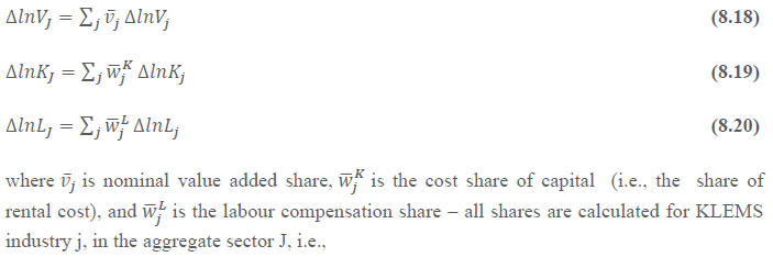  where PV,j is the price of value added in industry j, Vj is the real value added in industry j, PK,j is the rental price of capital in industry j, Sj is the capital stock in industry j, PL,j is the wage rate (price of labour) in industry j, and Hj is the employment in industry j. The aggregate output and input growth rates obtained above are then used with the growth accounting equation to obtain the sectoral TFP growth rates (see equation 8.3; an equation similar to that equation is used in which only value added, labour input and capital input are considered along with the income shares of labour and capital in gross value added). 1 Timmer, M.P, Mahony, M. and van Ark, B. (2007). The EU KLEMS growth and productivity accounts: an overview. Mimeo University of Groningen & University of Birmingham, 2 Readers can refer to India KLEMS Data Manual Version 2013 for the data set released by RBI on its website in June 2014. 3 The difference between value added at factor cost and value added at basic price is the treatment of taxes and subsidies on production. While the former excludes all taxes on production and includes all subsidies (on intermediate inputs and factor inputs), the latter includes only taxes and subsidies on intermediate inputs. In practice, gross value added at basic prices is measured as output valued at basic prices less intermediate consumption valued at purchasers' prices. The basic price is the amount receivable by the producer from the purchaser for a unit of a good or service produced as output minus any tax payable, and plus any subsidy receivable, on that unit as a consequence of its production or sale. It excludes any transport charges invoiced separately by the producer. Although the outputs and inputs are valued using different sets of prices, for brevity the value added is described by the prices used to value the outputs. From the point of view of the producer, purchasers' prices for inputs and basic prices for outputs represent the prices actually paid and received. Their use leads to a measure of gross value added which is particularly relevant for the producer. 4 From both aggregated 9 NAS sectors Gross Domestic Product by economic activity statement along with the disaggregated statements of these 9 NAS sectors. 5 Refer to Appendix B for details about all the employment and unemployment surveys conducted by NSSO in India. 6 This procedure has been advocated by NSSO itself and has been consistently adopted by almost all researchers. 7 A very lucid description of the same is given by Sivasubramonian (2004). 8 The 66th round has not been used because of its inconsistency with the 61st and 68th round. Most economists consider it as an outlier. 9 Refer to Appendix C for detailed definition of UPSS, CWS and CDS. 10 Problems in using UPSS are: The UPSS seeks to place as many persons as possible under the category of employed by assigning priority to work; no single long-term activity status for many as they move between statuses over a long period of one year, and Usual status requires a recall over a whole year of what the person did, which is not easy for those who take whatever work opportunities they can find over the year or have prolonged spells out of the labour force. 11 Appendix Table D provides the details for the four segments about the Census Population, WFPR by UPSS, and persons employed in each of the EUS rounds used in the study. 12 Aggregate input is measured as a translog index of its individual components. Then the corresponding index is a Törnqvist volume index (see Jorgenson, Gollop and Fraumeni 1987). For all aggregation of quantities, we use the Törnqvist quantity index, which is a discrete time approximation to a Divisia index. This aggregation approach uses annual moving weights based on averages of adjacent points in time. The advantage of the Törnqvist index is that it belongs to the preferred class of superlative indices (Diewert 1976). Moreover, it exactly replicates a translog model which is highly flexible, that is, a model where the aggregate is a linear and quadratic function of the components and time. 13 The assumption basically requires perfect competition in labour market, which does not exist in countries like India. It thus restricts the applicability of such a method in situations where there may be widespread monopsony power or bilateral monopoly within an industry. 14 EU KLEMS faces this problem by restricting the estimation of change in labour quality in some cases to only fifteen aggregate industries and assuming it to be same for sub-industries (Timmer, et al; 2010; p 118). 15 The index can also be described as “education” index, as only educational characteristic has been used in its computation. 16 In EU-KLEMS changes in labour quality have been measured by including employment class, gender, age and education (Timmer, op cit.; p.64) and only 3 categories of education, defined as high skilled, medium skilled and low skilled have been taken. This concept of labour quality is refereed as ‘labour quality’ by Jorgenson. It is recognized (Timmer, et.al.; op cit; p84) that the categorization may lead to biases in the aggregate quality adjustment if employment trends and wage share differ within categories. These education categories generally correspond to- up to Primary education, above Primary to Hr. Secondary education and above Hr Sec or College education. Since due to data limitations, we have measured changes in labour quality only by changes in education profile of labour therefore, it became desirable to have a more detailed classification of education to capture the changes in skill quality of Indian workers. 17 In PLFS (2017-18), the earnings by self-employed are also provided, but for consistency with other rounds we have used the same procedure of Mincer equation even for this round. In EU KLEMS (Timmer, et.al., op cit; p 67) it is assumed that the earnings of the self-employed is equal to the earnings of ‘regular' employees. 18 The details of the function can be obtained from the Stata software and are also provided in Box 1. 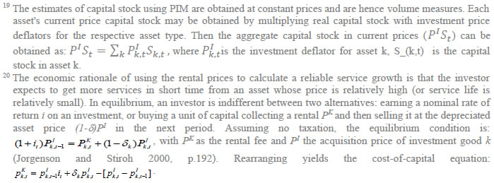 21 This version of the database does not make a distinction between ICT and non-ICT assets, as the industry level data on ICT assets are weak. An attempt to estimate aggregate economy level ICT capital can be found in Erumban and Das (2015). 22 See O’ Mahony and Timmer (2009) for a description of EU KLEMS database 23 This data is not publicly available. However, CSO has been kind to compile this data for the India-KLEMS project. 24 In some years transport equipment was provided as part of the machinery and equipment, categorized as ‘tools, transport equipment and other fixed assets. In such cases, we use transport/tools, transport and other fixed asset ratio in the nearest year to separate transport equipment. 25 This choice is driven by the fact that the first year of availability of ASI data is 1964-65. 26 National Accounts Statistics-Sources and Methods, Chapter 26, CSO (2007), 27 We do not intend to delve into the controversies over the use of internal vs. external rate of return in the context of productivity measurement. This database uses See Erumban (2008a and b) for a discussion on these issues. 28 Reserve Bank of India, Handbook of Indian Statistics, Annual volumes. 29 IOTT 2015-16 was published by Brookings India. 30 The estimation is done at group level rather than individual industries on the consideration that the group level estimates will be more reliable. 31 Consider, the semi-conductor (SC) industry, which is a key input to the computer hardware industry. Much of the output is invisible at the aggregate level because semi-conductor products are intermediate inputs to other industries rather than deliverables to final demand - consumption and investment goods. Moreover, SC plays a role in the improvements in quality and performance of other products like-computers, communication equipments and scientific instruments. Failure to account for them leads us to miss the role of key industries that produce intermediate inputs and importance of intermediate inputs for the industries that use them. (Jorgenson, Ho and Stiroh (2005), Productivity, volume 3). |
||||||||||||||||||||||||||||||||||||
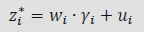

Measuring Productivity at the Industry Level - The India KLEMS Database
|
AUTHORS Sadhan Kumar Chattopadhyay Director Siddhartha Nath Assistant Adviser Sreerupa Sengupta Manager Shruti Joshi Manager
This document describes the procedures, methodologies and approaches used in constructing the India KLEMS database version 2021. Till now, the work relating to compilation of India KLEMS data was being done by the India KLEMS team housed at the Centre for Development Economics, Delhi School of Economics. Now the work has been shifted to the KLEMS Division of Department of Economics and Policy Research of RBI since February 2021 and hence the KLEMS data have been compiled independently by the KLEMS Division under the supervision of India KLEMS team. This work is meant to support empirical research in the area of economic growth. In addition, the database is meant to support the conduct of policies aimed at supporting acceleration of productivity growth in the Indian economy, requiring comprehensive measurement tools to monitor and evaluate progress. Finally, the construction of the database would also support the systematic production of reliable statistics on growth and productivity using the methodologies of national accounts and input-output analysis. Following the earlier trend, this version of database includes measures of economic growth, employment creation, capital formation and productivity at the industry level from 1980-81 onwards. The input measures will incorporate various categories of Capital (K), Labour (L), Energy (E), Materials (M) and Services (S) inputs. The present document describes the India KLEMS database version 2021. In fact, the present version is an extended India KLEMS research project, “Disaggregate Industry Level Productivity Analysis for India- the KLEMS Approach” undertaken at the Centre for Development Economics, Delhi School of Economics. The dataset includes measures of Gross Value Added (GVA), Gross Value of Output (GVO), Labour (L), Capital (K), Energy (E), Material (M), Services (S), Labour Quality (LQ), Labour Productivity (LP) and Total Factor Productivity (TFP) at the industry and economy level from 1980-81 onwards. The database covering the period 1980-81 to 2019-20 has been constructed on the basis of data compiled from NSO, NSSO, ASI, Input-Output tables (I-O tables) and processed according to appropriate procedures. These procedures were developed to ensure harmonization of the basic data, and to generate growth accounts in a consistent and uniform way. Harmonization of the basic data has focused on several areas such as industrial classification, and aggregation levels. The data base covers 27 industries comprising the entire Indian economy. The industries are shown in Table 1.1 below. The variables in the data set are given in Table 1.2. 1.2 Coverage: Industries and Variables In this section we describe the coverage of the India KLEMS database in terms of industries and variables. In principle, the 39-year period from 1980-81 (1980) to 2019-20 (2019) is covered. At a disaggregated level, database is created for 27 industries. The industrial classification is constructed by building concordance between NIC 2008, NIC 2004, NIC 1998, NIC 1987 and NIC 1970 to generate continuous time series from 1980 to 2019. This classification is very close to the International Standard Industrial Classification (ISIC) revision 3. The 27 industries are aggregated to form six broad sectors, namely:
Table 1.1 provides a listing of the 27 industries, including the higher aggregates. For detailed classification and concordance of study industries with NICs, readers may refer to Version 7 of the manual published in 2021. Table 1.2 provides an overview of all the series included in our database. Measures of Capital (K), Labour (L), Energy (E), Material (M) and Service (S) inputs as well as Gross Output (GO), have been constructed using National Accounts Statistics (NAS), Annual Survey of Industries (ASI), NSSO rounds and Input-Output (IO) Tables. In building annual time series on gross output, five inputs and factor income shares, various assumptions are made to fill up gaps in industry details and link series over time. As we know that NSSO rounds of unregistered manufacturing, Input Output Transaction Tables, and Employment and Unemployment Surveys by NSSO are available only for certain benchmark years. The use of information from these data sources necessitates interpolation and assumption of constant shares for building series of output and inputs. Further the construction of growth accounting series like total factor productivity, labour productivity, etc. are based on theoretical models of production and needs additional assumptions that are spelt out in subsequent chapters of the manual. Finally, the other Series like NDP at factor cost, compensation of employees, etc. are additional series which are used in generating the growth accounts and are informative by themselves. Chapter 2: Gross Value-Added Series at the Industry Level This chapter describes the data sources and methodology used to construct the Gross Value Added (GVA) series at current and constant prices for 27 study industries for the period of 1980-81 (1980) to 2019-20 (2019). The National Accounts Statistics (NAS) brought out by the NSO (National Statistics Office, Government of India) is the basic source of data for the construction of series on gross value added for INDIA KLEMS-industries. Up to 2011-12, estimates of GVA at both current and constant (2011-12) prices for all industries are obtained from Back Series of National Accounts (Base 2011-12). For years after 2011-12, they are directly obtained from NAS 2022. However, NAS estimates of value added are not available for a few India KLEMS industry groups. Therefore, we had to split some of the aggregate industry groups from NAS. Maintaining consistency with NAS, the value-added data in India KLEMS is measured at basic price. The construction of Gross valued added series involves three steps. Step 1: A concordance table between the classification used in the NAS and the 27 study industry classification used for this project has been prepared. Further, concordance between all the 27 sectors has been constructed with NIC- 1970, 1987, 1998, 2004 and 2008. Out of the 27 study industries, for 20 industries, GVA series both in current and constant prices is directly taken from NAS1. The sectors for which data are provided in NAS are Agriculture, Forestry & logging, Fishing, Mining and Quarrying, Manufacturing, Electricity,gas and water supply, Construction, Trade, Hotels & Restaurants, Railways, Transport by other means, Storage, Communication, Banking & insurance, Real estate, Ownership of Dwelling & Business Services, Public Administration & Defense and Other Services. Step 2: For manufacturing industries where direct estimates of GVA were not available from NAS, estimates have been made using additional information from ASI and NSSO unorganized manufacturing data. In these cases, GVA data is constructed by splitting the NAS data using ASI or NSSO distributions. ASI data (annual) has been used for registered and corporate manufacturing whereas interpolated ratios from NSSO 40th (1984-85), 45th (1989-90), 51st (1994-95), 56th (2000-01) 62nd (2005-06), 67th round (2010-11) and 73rd round (2015-16) rounds have been used for Unregistered and household manufacturing segments. For unregistered manufacturing for years 2015-16 to 2019-20 the ratio obtained from 73rd round of unregistered manufacturing has been used for the splitting. Table 2.1 and 2.2 showcases the methodology used to split GVA of certain NAS sectors to match concordance with our classification. It is important to note that the industry level value added volume indices are based on NAS. NSO provides single deflated value-added estimates for all sectors except Agriculture. Step 3: According to India KLEMS, GVA is adjusted for Financial Intermediation Services Indirectly Measured (FISIM). The details method of FISM adjustment is provided in earlier versions of KLEMS manual. Chapter 3: Gross Output Series at the Industry Level This chapter describes the procedures and methodologies used in constructing the database for gross output series at the industry level over the period 1980-81(1980) to 2019-20(2019). To construct the gross output series at industry level, we use multiple data sources namely National Accounts Statistics, Annual Survey of Industries, NSSO rounds for unorganized manufacturing and Input Output Transaction tables. The data sources and methodology used are documented below: National Accounts Statistics: The NAS is the basic source of data for the construction of time series on the gross output. The NAS back series 2011 with base 2004-05 and NAS 2014 provides estimates of gross output for six disaggregate industries at current and constant prices since 1950-51 till 2011-12. These sectors are Agriculture, Mining and Quarrying, Construction and Manufacturing sectors (Registered and Unregistered Manufacturing). However, the Back Series with base 2011-12, which is the source of GVA in India KLEMS database 2021, does not provide estimates of GVO for most of the industries except for Agriculture, Mining and Quarrying and Construction. For these three industries GVO data at current and constant prices directly obtained from Back Series with base 2011-12. Therefore, for 1980-81 to 2011-12 period, we estimate the GVO series for remaining 24 industries at current and constant prices by applying the respective GVO/GVA ratio for current and constant prices obtained from Back Series with base 2004-05 and NAS 2014 to GVA with 2011-12 base. For years since 2011, we take the estimates of GVO both at current and constant prices for all industries directly from NAS 2022. (a) Filling procedures of National Accounts series: It is to be noted that the NAS estimates of gross output for a few industry groups are at a more aggregate level, requiring splitting of the aggregates. In such cases, NAS estimates of output have been split using additional information from Annual Survey of Industries and NSSO rounds of Unregistered Manufacturing to obtain estimates at higher level of disaggregation. Secondly, for Unregistered manufacturing gross output data is available in NAS from 2004-05 onwards. In this case, information from NSSO survey rounds has been used for missing years to derive output estimates of unregistered manufacturing industries at current and constant prices. As mentioned earlier, for gross value-added series of service sectors we obtain our estimates from NAS. However, prior to 2011-12 National Accounts do not provide any estimates of gross output of service sectors and hence we rely on Input output transaction tables (from which the ratio of gross to value added is computed which is then applied to GVA reported in NAS) which are available at an interval of 5 years or so. This necessitates interpolation and assumption of constant shares for measuring output of services sectors. The Input Output Transaction Tables for Benchmark years of 1978-79, 1983-84, 1989-90, 1993-94, 1998-99, 2003-04 and 2007-08 are used to derive gross output series for service sectors. The construction of the gross output series at current and constant prices involves the following steps: Step 1: Measuring Gross Output of Agricultural Sector, Mining and Quarrying, and Construction NAS provides nominal and real GVO series for a) Crops and Plantation, b) Animal Husbandry c) Forestry and Logging d) Fishing. By aggregating the GVO of these four subsectors we derive the GVO of Agricultural sector. The Gross output estimates of Mining and Quarrying and Construction at current and constant prices from 1980-2019 is also directly taken from NAS. Step 2: Measuring Gross Output of Manufacturing Industries Since 2011-12, gross output data for 7 out of 13 manufacturing industries listed in table 3.1 are directly picked up from NAS. For the remaining 6 sectors output is constructed by splitting the NAS output data using ASI or NSSO distributions. ASI data (annual) has been used for registered manufacturing whereas interpolated ratios from 67th (2010-11) and 73rd (2015-16) rounds have been used for Unregistered Manufacturing segments. A list of study industries is presented in Table 3.2 showcasing the methodology used to split GVO of certain NAS sectors to match concordance with our classification for the year 2011 to 2019. Step 3: Measuring Gross Output for Services Sectors and Electricity, Gas and water supply Since 2011-12 NAS provided estimates of GVO at current and constant prices. Prior to 2011-12 Gross Output series for Services sectors and sector Electricity, Gas and Water supply have been constructed using information from Input – Output Transaction Tables of the Indian economy published by CSO. The details method of construction of GVO back series for services is provided in earlier versions of KLEMS Data manual. Chapter 4: Labour Input Series at the Industry Level This chapter provides information on the sources of data and method of measuring labour services. The aim is to estimate labour input so that it reflects the actual changes in the quantity (number of persons) and quality of labour input over time. The section discusses the construction of labour input for 27 industries from 1980 to 2019-20. Labour input is measured by combining data on labour persons and data on labour quality which is measured in terms of human capital embodied in the labour. In our study, we measure this on the basis of the educational qualification of the worker. It is important to segregate labor employed from labor quality because the contribution to output by each person also comes from this embodied capital. Moreover, the reward (wages and earnings) to each person also includes the reward for investment in human capital. Therefore, it is essential to separate out these differences in labour to clearly understand the underlying differences in labour characteristics. It is in this context that an endeavor has been made to estimate labour quality index. However, given the limitations of India’s employment statistics (Sivasubramonian; 2004, & Himanshu; 2011, Ghose; 2016), especially the availability of information on wages/ earnings of different category of workers which could be used as an indication of their differences in ability makes it difficult to quantify these changes in the labour force in a pertinent way. Therefore, the study has computed the labour quality index based on five different education categories only. This study aims to build a time series of employment and labor quality series for 27 industrial sectors. In this section we outline the sources of data and the methodology used. The section develops and implements the methodology of estimating persons employed (employment) and labour quality and combining the two to obtain the indices of labour input. Sources of data The Employment and Unemployment Surveys (EUS) of major rounds from 38th round (1983) to 68th round (2011-12) by National Sample Survey Office (NSSO) and the Periodic Labour Force Surveys (PLFS) of 2017-18, 2018-19 and 2019-20 by National Statistical Organization (NSO) are the main sources for estimating the total workforce in the country by industry groups, as per the National Industrial Classification (NIC). This year the study has adjusted the employment estimates obtained from Economic-Survey 2021-22 (pp.371). Methodology The employment in India has been computed in a step-wise manner as follows: As a first step concordance between the KLEMS 27 sectors, and NIC-1970, 1987, 1998 and 2008 was done. Thereafter, the following steps were done:
For extrapolation backward to 1980-81 to 1982-83, the interpolation of the broad industrial classification of 32nd round (1977-78) and 38th round (1983-84) is used. Thus, the estimates from 32nd round are mainly used as control numbers. Between 2005 and 2011, we observed very high growth rate in number of employed persons series for the industry Electrical and Optical Equipment as compared to other manufacturing industries and the overall growth in employment in this industry during 2005-2011 was found to be higher than that for Construction (which seems somewhat unrealistic). It was also observed that there was a negative growth in employment in Textiles, Textile Products, Leather and Footwear although real GVA of this industry more than doubled between 2005 and 2011. To address these issues, some adjustments to the initial employment estimates for Electrical & Optical Equipment and Textiles, Textile Products, Leather and Footwear have been done. Onwards 2005, employment series for Electrical & Optical Equipment has been estimated applying annual growth rates obtained from ASI and NSSO rounds to the number of employed persons for the year 2005-06. Then, for the years 2005-06 to 2011-12, we compute the difference between estimated employment series from EUS rounds and that based on ASI & NSSO rounds for the Electrical and Optical Equipment industry and add it to Textiles, Textile Products, Leather and Footwear industry. This ensures that for the manufacturing as a whole our estimates remain the same as obtained from EUS rounds. (b) Measuring quality index The quality of labour force is of considerable importance in the context of productivity measurement, and one of the widely used methodologies to capture changes in labour quality is given by Jorgenson, Gollop and Fraumeni (JGF) (1987). In growth accounting methodology of measurement of total factor productivity (TFP) when output growth is decomposed into growth of inputs and the residual TFP, then labour input is measured as an index of labour service flows. It accounts for changes in labour quality in terms of labour characteristics such as educational attainment, age (experience), gender, employment status, etc. and thus accounts for heterogeneity of the labour force. In our study, the index of aggregate labour quality measures the changes in the composition of labour in the economy. The present study has computed labour quality index by using only education characteristic in the JGF methodology. Thus, the data required for the labour quality index in the present case, is employment and earnings by education and by industry. The labour quality index has been computed using five education categories namely- up to primary, primary, middle, secondary & higher secondary, and above higher secondary. There are thus five types of persons employed for each of the 27 study industries. The quality growth rates are estimated for total persons employed in these industries in India for the 38th, 50th, 55th, 61st, 68th and PLFS rounds of NSO. They are then indexed to 1983 (38th round) as the base, so as to assess the temporal changes in labour’s skill and interpolation has been done between the major rounds for values of the intermediate years. Since the series is required from 1980-81, we have extrapolated it backwards from 1983 and the index is recomputed with base 1980-81 equal to 100. Therefore, the following steps have been performed:
 The first term of equation 4.1 indicates the changes in labour quality index, which is due to the changes in the composition of workers and the second term indicates the change in total persons employed in sector ‘j’. The index of aggregate labour quality thus measures the changes in the composition of labour in the economy The labour input (adjusted labour persons) then can be obtained by multiplying the number of persons employed by the corresponding labour quality index and the labour input growth is finally obtained by combining the growth of persons employed and the growth in the index of labour quality. Appendix A: Definitions of Employment in NSSO employment & unemployment surveys The surveys of NSSO on employment and unemployment (EUS) aim to measure the extent of ‘employment’ and ‘unemployment’ in quantitative terms disaggregated by various household and population characteristics following the three reference periods of (i) one year, (ii) one week, and (iii) each day of the week. Based on these three reference periods three different measures, termed as usual status, current weekly status, and the current daily status, are arrived at. While all these three approaches are used for collection of data on employment and unemployment in the quinquennial surveys, the first two approaches only are used for the purpose in the annual surveys. Usual principal status: In NSS 27th round, the usual principal activity category of the persons was determined by considering the normal working pattern, i.e., the activity pursued by them over a long period in the past and which was likely to continue in the future. For the identification of the usual principal status of an individual based on the major time criterion, in NSS 27th, 32nd, 38th, 43rd rounds, a trichotomous classification of the population was followed, that is, a person was classified into one of the three broad groups ‘employed’, ‘unemployed’ and ‘out of labour force’ based on the major time criterion. From NSS 50th round onwards, the procedure was changed and the prescribed procedure was a two-stage dichotomous one which involved a classification into ‘labour force’ and ‘out labour force’ in the first stage, and thereafter, the labour force into ‘employed’ and ‘unemployed’ in the second stage. Usual subsidiary status: In the usual status approach, besides principal status, information in respect of subsidiary economic status of an individual was collected in all employment and unemployment surveys. For deciding the subsidiary economic status of an individual, no minimum number of days of work during the last 365 days was mentioned prior to NSS 61st round. In NSS 61st round, a minimum of 30 days of work, among other things, during the last 365 days, was considered necessary for classification as usual subsidiary economic activity of an individual. Current weekly status: It is important to note at the beginning that in the EUS of NSSO, a person is considered as worker if he/she has performed any economic activity at least for one hour on any day of the reference week and uses the priority criteria in assigning work activity status. This definition is consistent with the ILO convention and used by most of the countries in the world for their labour force surveys. In NSSO, prior to NSS 50th round and in all the annual surveys till NSS 59th round, data on employment and unemployment in the CWS approach was collected by putting a single-shot question ‘whether worked for at least one hour on any day during the last 7 days preceding the date of survey’. The information so collected was used to determine the CWS of the individuals. This procedure was criticized for being not able to identify the entire workforce, particularly among the women. It was then decided to derive the CWS of a person from the time disposition of the household members for the 7 days preceding the date of survey. The procedure was used for the first time in NSS 50th round. It is seen that the change in the method of determining the current weekly activity had resulted in increasing the WPR in current weekly status approach - more so for the females in both rural and urban areas than for males. The trend observed in NSS 50th round in respect of the WPR according to CWS suggested continuing with the procedure for data collection in CWS in NSS 55th and NSS 61st rounds. Current Daily Status Current Daily Status (CDS) rates are used for studying intensity of work. These are computed on the basis of the information on employment and unemployment recorded for the 14 half days of the reference week. The employment statuses during the seven days are recorded in terms of half or full intensities. An hour or more but less than four hours is taken as half intensity and four hours or more is taken as full intensity. An advantage of this approach was that it was based on more complete information; it embodied the time utilisation, and did not accord priority to labour force over outside the labour force or work over unemployment, except in marginal cases. A disadvantage was that it related to person-days, not persons. Hence it had to be used with some caution. Chapter 5: Capital Input Series at the Industry Level This chapter outlines the methodology employed to estimate capital input for the 27 industries in the India KLEMS database version 2022. All the productivity calculations in India KLEMS use capital services as an input to production, which is estimated using the approach developed by Jorgenson and Griliches (1967), and outlined in Jorgenson, Gollop, and Fraumeni (1987). The estimation of capital service growth rates is accomplished by first estimating capital stock for different capital assets, and then aggregating across assets after correcting for the differences in their marginal productivities. Capital services account for the differences in marginal productivity between different asset types while capital stock measures only the vintages of capital, they do not account for asset heterogeneity. For instance, aggregate capital stock measures would assume that a computer's productivity is the same as that of a car. However, proper measures of capital stock would account for the decline in the efficiency of both computers and cars over their lifetime. Following an overview of the theoretical method to measure capital services (Jorgenson and Griliches,1967; JGF, 1987), the chapter discusses the specific empirical approaches we follow to implement these methods within the constraints of data availability for Indian industries. In India KLEMS, we have reported capital stock, capital services and the capital “capital composition effect”. Capital stock is reported in constant price volumes, and growth rates, while the latter two are reported in growth rates and indices. To measure capital services, using the Jorgenson and Griliches (1967) approach, we need estimates of capital stock for detailed asset types and the shares of each of these assets in total capital remuneration. The aggregate capital services growth rate is derived as a weighted growth rate of individual capital assets, the weights being the shares of each asset in the total compensation made to capital, i.e, 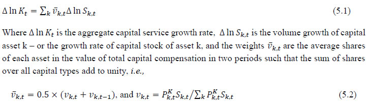 where PKk,t is the rental or user cost of capital asset type k in year t. Therefore, the numerator, which is the product of user cost of asset k and the capital stock of asset k, is the capital compensation received by asset k. The numerator is the sum of compensation received by assets, or the total capital compensation, and therefore vk,t is the share of asset k in total capital compensation. Under the neoclassical assumption of price-marginal product equality, it effectively incorporates the productivity or qualitative differences in the contribution of various asset types to aggregate capital services, as the composition of aggregate capital stock in any industry changes (see Jorgenson, 2001). For instance, as the marginal productivity of ICT capital is higher than that of other assets, a change in the composition of capital towards ICT capital will result in higher capital services, which will be captured by a larger value of the v for ICT assets. It is evident from (5.2) that two important components of capital service measure are the asset wise capital stock, Sk,t and the service price (rental price) of capital assets, PKk,t. Assuming a geometric depreciation rate, δk which is constant over time, but different for each asset type, capital stock in asset k in year t can be constructed using Perpetual Inventory Method (PIM) as:7  where, Ik,t is the real investment in asset type k in period t. For a detail discussion on PKk,t, please see Box 5.1A in the Appendix B. 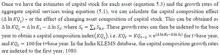 Since our measure of capital input takes account of asset heterogeneity, it was essential to obtain investment data by asset type. We distinguish between 3 different asset types – construction, transport equipment, and machinery (includes ICT and non-ICT machinery).8 We exploit multiple sources of information for the construction of our database on capital services. This includes the National Accounts Statistics (NAS) that provide information on broad sectors of the economy, the Annual Survey of Industries (ASI) covering the organized manufacturing sector, the National Sample Survey Office (NSSO) rounds for unorganized manufacturing and various Input-Output tables. Even though we use multiple sources of data, our final estimates are fully consistent with the aggregate data obtained from the NAS. In addition, our approach to capital measurement is consistent with international practices such as the EU KLEMS9, which ensures the possibility of international comparisons. In what follows, we discuss the various sources of data for asset wise investment and the construction of the relevant variables, in detail. (a) Asset-wise investment for broad sectors of the economy Industry-level estimates of capital input require detailed asset-by-industry investment matrices. NAS provides information on aggregate capital formation by industry of use for nine broad sectors, which, nevertheless, was not sufficient for our purpose. Therefore, we have collected more detailed data on assets and industries from the CSO.10 This is the data underlying the published aggregate gross fixed capital formation by the broad industry groups, separately for public and private sectors. For those sectors for which the investment matrices were not available from CSO, we gather information from other sources (e.g. ASI for organized manufacturing and NSSO surveys for unorganized manufacturing) and benchmark it to the aggregate investment series from the National Accounts. The data used in the current version of the India KLEMS is based on the revised NAS with 2011-2012 base and is available only since 2012. Therefore, for earlier years, we extrapolate the series using growth rates from previous version of the data. Table 5.1 provides an overview of asset types available in NAS and their corresponding asset types used in our study. Investment in education and health are obtained directly from national accounts for the period after 2012, for each asset. For years before 2012, we assume the trend in the distribution of output, in order to split the total investment in the aggregates of these sectors into sub-sectors.
Total investment in each asset category is calculated as the sum of private and public sector investment in each asset. Investment in transport equipment was not available separately for the private sector industries. Therefore, we distributed the NAS total machinery in the private sector using the industry distribution of machinery and transport equipment. These estimates are then subtracted from each industry’s total machinery & transport equipment data to obtain the transport equipment investment in the private sector industries. Using this approach, we could generate investment in transport equipment by industries for the period 1950-2016. We assumed the share of transport equipment in the total machinery and equipment group in 2016-2017 to remain constant to create nominal investment in transport equipment in the subsequent years. The nominal investment was deflated using GFCF deflator for transport equipment (see section (c)). Since the distinction between registered and unregistered manufacturing is not available in the NAS since 2016, we used a quick fix to split these two. NAS provides a division between the corporate sector, public sector, and household sector. In the current version of the data, we consider the household sector as a proxy for unregistered and the corporate and public sector as a proxy for the registered sector. As mentioned earlier, the updates for years since 2017-2018 are solely based on published aggregate GFCF data from the National Accounts. In the 2019 version of the India KLEMS, we considered the 2012-2016 detailed asset-wise data by industries provided by the CSO as such and extended the data for 2017-2018 using the published aggregates. However, in the 2020 version of the data, we changed this approach, as there were some discrepancies between the published NAS totals and the detailed asset-industry data. While extending the past series of detailed asset-wise investments forward for years since 2017-2018 using the NAS-published headline series, we now consider the published NAS series as the benchmark since 2012. Then we apply the industry distribution of the 2012-2016 detailed series obtained previously from the CSO. The current approach is more appropriate and ensures a complete consistency with the NAS-published series. However, it may cause some changes in the capital service growth rates compared to the last release12. (b) Asset-wise investment for non-NAS sectors NAS provides data only for 9 broad sectors, while we have 27 industries, which necessitated further splitting of some of the NAS sectors. This includes aggregate manufacturing (registered and unregistered separately for the period 1950-2016) with 13 sub sectors; other services into 4 sub sectors; and real estate activities and business services into 2 sub sectors. The manufacturing sector investment data was disaggregated into 13 subsectors at the 2-digit level of NIC 1998 using ASI and NSSO data, which will be discussed in detail subsequently. Investment series in service sector has been split into sub sectors using two alternative approaches–value added shares, and capital/labour ratio in the higher aggregate industry. However, the final data used are based on value added shares, as we did not see any significant difference between the two. Registered (organized) Manufacturing: In order to split the aggregate capital formation in organized manufacturing sector into 13 study sectors, we use the ASI. ASI defines GFCF as actual additions (newly purchased, second hand and own construction) minus deductions plus depreciation adjustment for discarded assets during the year. This approach is based on a single year’s sample and helps to avoid potential huge negative investment series, and is also consistent with published ASI GFCF series. The yearly detailed volumes beginning 1964-65 were used to derive the gross fixed capital formation by asset type directly. For the years 1964-1978, the relevant data are obtained from published detailed volumes. For the period, 1983-84 to 2004-05 ASI has generated detailed tables from Block C of ASI schedule that contain data on fixed assets. Data for missing years are interpolated using the changes in investment using book value method13. Table 5.2 provides an overview of the asset categories available in ASI, and the relevant asset categories in our study to which they are attributed. Though ASI provides investment in land, for reasons of NAS consistency we exclude it from our database. Once investment in each of these assets and industries are generated using ASI data, we apply this industry-asset distribution to the published aggregate NAS GFCF series for organized manufacturing sector. It may also be noted that from 1960-61 to 1971-72, ASI data are for the census sector and from 1973-74 onwards they are for the factory sector. In order to make these two series comparable over years, we convert the data prior to 1972 to factory sector using the factory/census ratio in 1973. Thus, after these adjustments, we obtain investment data for 13 manufacturing sectors, by asset types, consistent with the NAS aggregate for registered manufacturing. This approach was accurate for the period 1950-2016 when the NAS provided aggregate registered manufacturing GFCF data. For the years after 2016, since when NAS does not provide registered manufacturing aggregate, we proxy registered manufacturing by the sum of public sector and corporate sector. Unregistered (unorganized) Manufacturing: The data required for creating the gross investment series for the 13 sectors of the unorganized manufacturing sector are obtained from various rounds of NSSO surveys on unorganized manufacturing. We use 6 rounds of NSSO surveys that cover the period 1989-2016. These are 45th round (1989-90), 51st round (1994-94), 56th round (2000-01), 62nd round (2005-06), 67th round (2010-11) and 73rd round (2015-16). Unit level data has been aggregated to 13 industries using the appropriate concordance. NSSO provides net addition to owned assets during the reference year within the block of fixed assets, and we use this as a measure of our investment. The investment series arrived at for six rounds were interpolated to obtain the annual time series of unorganized gross fixed capital formation by asset type. As in the case of registered sector, once the investment by asset types across industries are constructed, the asset-industry distribution is applied to the published NAS aggregate GFCF in unregistered manufacturing to obtain NAS consistent GFCF by asset type and industries. (c) Investment Prices by Asset Types In order to compute asset wise capital stock using PIM (equation 5.3) and rental price (see Box 5.1A in the Appendix), we require asset wise investment price deflators. Since CSO has provided us with investment data by industries and assets both in current and constant prices, we could derive the price deflators with base 2011-2012. For years before 2011, prices were spliced using 2004-2005 base investment deflators. These deflators are directly used for all the three asset categories we have. Since there was no separate asset wise data available for transport equipment in 2017-2018, the investment deflator for transport equipment from 2016-2017 was extrapolated using the trend in the investment price of total machinery & equipment, obtained from NAS. (d) Initial Stock, Depreciation Rates and Rate of Return For the implementation of PIM to estimate asset wise capital stock, we require an estimate of initial benchmark stock (see Erumban, 2008b for an in-depth discussion on this issue). NAS provides estimates of net capital stock since 1950 for all the broad sectors in its Statement 17: Net Fixed Capital Stock by industry of use. We take the NAS estimate of real net capital stock in 1950 (in 1999-2000 prices) as our benchmark stock for all non-manufacturing sectors, and for manufacturing sectors the same is taken for the year 1964.14 However, since the NAS estimate is available only for broad sectors and for aggregate capital, we use our industry-asset distribution of GFCF in order to create net fixed capital stock estimates by asset type for all the 27 sectors. The approach to split asset-wise capital stock is changed in the 2020 version of the India KLEMS database. Instead of using the GFCF distribution, we use the distribution of net capital stock by assets, available from the detailed asset data obtained from the CSO. Since the initial stock depreciates over the years, the impact of this change in distribution on the capital stock will vanish over the years at the individual asset level. However, as it changes the distribution of assets in the total capital stock, these compositional changes tend to have a visible impact on the aggregate capital stock, causing a historical revision of capital stock growth rates in some industries (esp. transport and storage, education, hotels and restaurants, electricity, transport equipment, etc.). NAS also provides detailed tables on assumed life of assets used for computing capital stock, for private units, administrative units as well as departmental and non-departmental units by asset types.15 We use these estimates of lifetime to derive appropriate depreciation rates for non-ICT assets, using a double declining balance rate. Following the NAS, we assume 80 years of lifetime for buildings, 20 years for transport equipment, and 25 years for machinery and equipment (see Appendix 26.2; CSO, 2007). The final depreciation rates used in the study are given in Table 5.3 by asset type. Subsequently, we build our capital stock series by asset types for all the 27 industries using our GFCF series from 1950 (1964) onwards for the non-manufacturing (manufacturing) sectors. Our measure of capital input is arrived using equation (5.1), for which we also require estimates of rental prices (see Box 5.1A in the Appendix). Assuming that the flow of capital services is proportional to the capital stock at individual asset level, aggregate capital flows can be obtained using a translog quantity index by weighting growth in the stock of each asset by the average shares of each asset in the value of capital compensation, as in (5.1). The rate of return (i) in equation (5.4) represents the opportunity cost of capital, and can be measured either as internal (or ex post) rate of return, or as an external (ex ante) rate of return.16 The present version of the database uses an external rate of return, proxied by average of return on government securities and prime lending rate obtained from the Reserve Bank of India17. Therefore, we use a real rate, which is net of capital gain. Hence, the capital gain component in equation is excluded while estimating rental price using external rate of return, obtaining  Where r is the real rate of return, nominal interest rate adjusted for consumer price inflation rate. The consumer price indices (CPI) are obtained from IMF and World Bank. The measures of capital input available in India KLEMS are based on only three asset categories, construction, machinery, and transport equipment. Therefore, it does not consider the enormous and distinct role of ICT capital in contributing to productivity and growth. The absence of ICT estimates in the database is driven by insufficient data on investment in ICT assets, such as hardware, software, and communication equipment in the National Accounts. However, during recent years, NAS has extended its asset coverage to include software and ICT equipment. Erumban and Das (2016) have made some estimates for the aggregate economy using input-output tables for ICT equipment and relying on NAS for software investment. Similarly, Erumban and Das (2020) have made some initial estimates of ICT capital by industries, which still remains a challenging task. Nevertheless, now that more data is available from NAS, it is possible to explore this further, and future extensions of the database may explore this. Similarly, following the SNA 2008 guidelines, the NAS now provides estimates of intangible capital such as intellectual property and research and development (R&D), which may be a useful extension to the capital input database. Two additional challenges are arising since the new system of national accounts. The first is the lack of separate data on registered and unregistered manufacturing, which poses challenges in using ASI and NSSO data to split aggregate manufacturing data into 13 industry groups. Instead of the registered and unregistered split, CSO now provides a division between the household and corporate sectors. We currently address this challenge by considering the household sector as unregistered manufacturing and the sum of public and corporate sectors as a registered sector. The second challenge is the lack of separate data on transport equipment and machinery assets in the new series of national accounts, which follows United Nation's System of National Accounts (SNA)-2008. Although, for the time being, we adopt ad-hoc approaches to fix this, it cannot be adopted on a long-term basis, which might necessitate combining transport equipment and machinery to one single asset. Finally, as mentioned earlier, the debate on whether it is appropriate to use an external rate of return or an internal rate of return is unsettled in the literature. It may be worth exploring estimates of capital using the internal rate of return. Appendix B: Some Discussions on the Estimation of Capital Services
Chapter 6: Intermediate Input Series at the Industry Level In this section, we describe the basic approach we have used to derive the volume series of Intermediate Inputs namely –Energy input (E), Material input (M) and Services input (S). The methodology for measuring industry output, intermediate inputs and value added was developed by Jorgenson, Gallop and Fraumeni (1987) and extended by Jorgenson (1990 a). The cornerstone of this approach is a time series of input output (IO) tables which gives the flows of all commodities in the economy, as well as payments to primary factors. Following a similar approach as explained in Jorgenson et al. (2005, Chapter 4) and Timmer et al. (2010, Chapter 3), the time series on intermediate inputs for the India KLEMS project have been constructed. Definition of EMS: As in EU KLEMS, this study identifies three main categories of Intermediate inputs. They are classified as follows: 1. Energy Input 2. Material Input 3. Service Input The following five energy types (and products) have been classified as the Energy input: 1. Coal and Lignite 2. Petroleum products 3. Electricity; (for electricity used in the electricity sector, since there is a good amount of inter-firm sale and purchase of electricity, it has been treated as material rather than as energy) 4. Natural gas 5. Gas (LPG) The following fourteen input items have been classified as the Service input: 1. Water supply 2. Railway transport services 3. Other transport services 4. Storage and warehousing 5. Communication 6. Trade 7. Hotels and restaurants 8. Banking 9. Insurance 10. Ownership of dwellings 11. Education and research 12. Medical and health 13. Other services 14. Public administration All other intermediate inputs barring the above mentioned nineteen inputs are classified as material input. The methodology for computation of Intermediate Input Series for 27 Industries from 1980-2019 at current and constant prices is explained in steps. Step 1: Concordance is done between IOTT and study industries
Step 2: Obtaining estimates for Material, Energy and Service Inputs for 27 Industries, in benchmark years 1. In IOTT, no intermediate input is being used in industry 24 – ‘Public Administration’. Consequently, the intermediate input series is being directly estimated for only 26 industries from 1980 to 2019. However, we have used ‘Net Purchase of Commodities and Services’ of Administrative Department as total intermediate input. And using information about ‘Government Final Consumption Expenditure’ we distribute the total intermediate input in to material, energy and services input. 2. Value of Energy Inputs used 3. Value of Material Inputs used 4. Value of Service Input used 5. Value of Total Intermediate Inputs (summation of the above three) Thus, for each of the benchmark year, estimates are obtained for Material, Energy and Service Inputs that has been used to produce Gross output in the 27 different India KLEMS Industries. Step 3: Projecting a time series (1980 to 2019) of proportions of Material, Energy and Service Inputs in Total Intermediate Inputs for each of the 27 industries
There exists some abnormal fluctuation in the proportions of Material Inputs, Energy Inputs, and Service Inputs in Total Intermediate Inputs for benchmark years. In that case, we drop that specific benchmark proportion and linearly interpolate of the adjacent benchmark proportions to estimate proportion for intervening years. For the industry ‘Wood & Wood Products’, we estimated proportions of Material Inputs, Energy Inputs, and Service Inputs in Total Intermediate Inputs from SUT 2015-16 instead of Input Output Transaction Table 2015-16. For the industry group ‘Coke, Refined Petroleum and Nuclear Fuel’, we estimated proportions of Material Inputs, Energy Inputs, and Service Inputs in Total Intermediate Inputs from ASI data instead of Input Output Transaction Table. This has been done because the relevant proportions differed significantly between the input-out tables and ASI, and the latter is believed to be making a more correct assessment of energy inputs used in the Coke and Petroleum products industry. Step 4: Consistency with NAS The projection of intermediate input vector, using IOTT in Step 3 needs to be consistent with the estimated output from NAS.
1. For Benchmark years: Ratio of Total Intermediate inputs from NAS to that from IOTT is adjusted proportionately to the absolute value of Energy Inputs/Material Inputs/Service Inputs obtained from IOTT. 2. For Intervening Years: The interpolated proportions of Energy Inputs, Material Inputs and Services Inputs obtained from IOTT, is applied directly to the total intermediate inputs from NAS to get each inputs share. Steps 1-4: This gives a time series of Material, Energy, and Service Inputs for 27 study Industries from 1980 to 2019 at current prices. Steps 5 and 6 below, explain the methodology for computation of Intermediate Input Series for 27 study Industries from 1980 to 2019 at constant price. The approach followed here is to first form the aggregates of materials, energy and services at current price for each study industry from the benchmark Input Output tables and then develop deflators of Materials, Energy and Service Inputs for each of the 27 study Industries separately. Step 5: Constructing Deflators of Materials, Energy and Service Inputs for 27 study Industries separately
Step 6: Computing Time Series on Intermediate Input for 27 study Industries from 1980-2019, Constant prices
Thus, we have a time series of Material, Energy and Service Inputs for 27 study Industries at constant prices. Chapter 7: Factor Income Share Series at the Industry Level The distribution of income between capital, labour and intermediate inputs, is an important element in growth accounting because income shares, under conditions of competitive markets, can be used to measure the contributions each factor makes towards output growth. 7.1 Methodology for Measuring Labour Income Share Series Under the assumption of constant returns to scale with two factors of production i.e., labour and capital, the sum of the labour income share and capital income share is 1. The labour income share is defined as the ratio of labour income to GVA. Capital income share is accordingly obtained as one minus labour income share. There are no published data on factor income shares in Indian economy at a detailed disaggregate level. National Accounts Statistics (NAS) of the CSO publishes the NDP series comprising of compensation of employees (CE), operating surplus (OS) and mixed income (MI) for the NAS industries. The income of the self-employed persons, i.e., mixed income (MI) is not separated into the labour component and capital component of the income. Therefore, to compute the labour income share out of value added, one has to take the sum of the compensation of employees and that part of the mixed income which are wages for labour. The computation of labour income share for the 27 study industries involves two steps. First, estimates of CE and MI have to be obtained for each of the 27 study industries from the NAS data which are available only for the NAS sectors (see Table 7.1). Second, the estimate of mixed income has to be split into labour income and capital income for each industry for each year (except for those industries for which the reported mixed income is zero, for instance, public administration). Basis data sources used for the computation of labour income share are NAS, ASI and unit level data of survey of unorganized manufacturing enterprises. These data sources are used to obtain estimates of CE, OS and MI for each of the 27 study industries. For splitting the labour and non-labour components out of the mixed income of self-employed, the unit level data of NSS employment-unemployment survey are used along with the estimates of CE, OS and MI basically obtained from the NAS. a) Construction of Labour Income Share Series in Gross Value Added The estimation of labour income share for the 27 study industries has been done in two steps, as discussed below. Step 1: Estimation of CE, OS and MI for the 27 study Industries NAS provides estimates of compensation of employees (CE), operating surplus (OS) and mixed income (MI) for the 9 NAS industries in different annual Sequence of National Accounts reports. For some industries under study, for instance (i) Agriculture, forestry & logging and fishing, (ii) Mining & Quarrying, (iii) Electricity, gas and water supply and (iv) Construction, the required data are readily available from NAS. For others, the estimates available in NAS have to be distributed across the study industries using ASI data. The NAS estimates of factor incomes (CE) for registered manufacturing is split into KLMES 13 industries (3-15) in proportion to the reported ASI data on emoluments for various industries. Estimate of factor incomes for ‘other services’ in NAS has been split into estimates for (i) Education, (ii) Health and Social Work, and (iii) Other Community, Social and Personal Services including Renting of Machinery and Business Services, and Private Household with Employed Persons. Before 2011-12, NAS provides estimates of factor incomes for registered manufacturing and unregistered manufacturing, but not for individual manufacturing industries. However, 2011-12 onwards NAS disaggregated the manufacturing sector in corporate sector and household sector. The NAS estimates of factor incomes for registered manufacturing and corporate sector have to be split into various manufacturing industries considered in the study (13 in number) using ASI data. The reported CE in NAS for registered manufacturing and corporate sector has been distributed into those 13 industries in proportion to the reported ASI data on emoluments for various industries. In a similar way, using ASI data, the estimate of OS for registered manufacturing and corporate sector has been distributed. Emoluments are subtracted from gross value added for various industries yielding capital income. The share of different industries in aggregate capital income of organized manufacturing indicated by the ASI data is used to split the estimate of OS for registered manufacturing and corporate sector reported in the NAS. The methodology applied for unregistered manufacturing and household sector is similar. The published results and unit level data of survey of unorganized manufacturing industries have been used for this purpose. The estimates of wage payments (to hired workers) in different industries have been used to split (proportionately) the estimate of CE in the NAS for aggregate unregistered manufacturing. The estimated wage payment is subtracted from the estimated value added to obtain an estimate of capital income and mixed income of the self-employed in various unorganized manufacturing industries. The estimate of MI provided in NAS for unregistered manufacturing and household sector has then been proportionately distributed across industries using the estimate of capital income and mixed income of the self-employed in various industries that could be formed on the basis of published results and unit level data of survey of unorganized manufacturing industries. Unlike the ASI data for organized manufacturing, the data for unorganized manufacturing enterprises are available for only select years. The proportions mentioned above could therefore be computed only for those select years (data for six rounds have been used; these are for 45th Round (1989-90), 51st Round (1994-95), 56th Round (2000-01), 62nd Round (2005-06), 67th round (2010-11) and 73rd Round (2015-16)). It has accordingly, been necessary to resort to interpolation/extrapolation to obtain the relevant proportions for other years. Step 2: Splitting of MI into Labour Income and Capital Income As explained above, the income share of labour is computed as:  In this equation, SLit is the labour income share in industry i in year t, CEit is compensation of employees in industry i in year t, MIit is mixed income of the self-employed persons in industry i in year t, and GVAit is gross value added in industry i in year t. The labour income proportion in income is denoted by η which taken to be a fixed parameter for each industry, not varying over time. The derivation of the GVA series for different industries has been briefly explained in Chapter 2. The derivation of CE and MI series has been explained in step I above. Therefore, only the estimation method of η needs to be described. The estimation of η has been done with the help of NSS survey-based estimates of employment of different categories of workers (number of persons and days of work) and wage rates (which has been described briefly in chapter 4) coupled with estimates of MI, basically obtained from the NAS. Two approaches have been taken to get an estimate of η, and the labour income share series for different industries finally adopted in the study makes use of an average of the estimates of η obtained by the two approaches. In the first approach, an estimate of labour income of self-employed workers has been made for each study industry for eight years, 1983-84, 1987-88, 1993-94, 1999-00, 2004-05, 2009-10, 2011-12 and 2015-16 on the basis of the estimated number of self-employed, wage rate of self-employed and the number of days of work per week. The industry-wise estimates of number of self-employed, wage rate of self-employed and the number of days of work per week have been made from unit records of NSS employment-unemployment survey (major rounds) of 1983, 1993-94, 1999-00, 2004-05, 2011-12, and PLFS of 2018-19 and 2019-20. The estimates of the number of self-employed, wage rate of self-employed and the number of days of work per week provide an estimate of the annul labour income of self-employed workers which is divided by the mixed income of self-employed (derived from NAS) to get an estimate of η. For five industries, the ratio in question has been computed and applied. For the other 22 industries, the ratio in question has been computed after clubbing the industries into 11 industry groups.19 In the latter case, a common ratio computed for group of industries has then been applied to constituent industries. The list of industries or industry groups for which η has been estimated is given in table 7.2. In the second approach, the NSS data are used to compute the following ratio: the ratio of labour income of self-employed workers to the labour income of regular and casual workers. Let this be denoted by θ. Then, the estimate of CE provided in the NAS is multiplied by θ to obtain an estimate of the labour income component out of the MI reported in the NAS. The labour component of MI divided by total MI gives an estimate of η. In case the estimated labour component of MI exceeds the estimate of MI, the estimate of η has been taken as unity. Examining the estimates obtained by the first approach, it was found that the estimated labour income share out of mixed income varied significantly among the estimates for the seven years for which the ratio in question has been estimated. The estimates of η obtained by the second approach has the problem that in a number of cases, the estimated labour component of MI exceeds the estimate of MI given in the NAS, and therefore η is taken as one. The method finally adopted is as follows: (a) The average value of η has been computed for each industry or industry group by taking the estimates for the years 1983-84, 1987-88, 1993-94, 1999-00, 2004-05, 2009-10, 2011-12 and 2015-16. This has been done separately for the estimates based on approach-1 and those based on approach-2. (b) The estimates of η obtained for each industry or industry group by the two approaches have then been averaged. (c) Having obtained an estimate of η, equation 7.1 given above has been applied to compute the labour income share. b) Construction of Factor Income Share Series in Gross output The income share of labour, capital and intermediate inputs in Gross output has been computed using the following steps:
The splitting of unorganized sector factor incomes into individual industries has been done using unorganized survey results. The proportions computed for 1983-84 has been applied for the period 1980-81 to 1983-84. While there were surveys of unorganized manufacturing enterprises in 1978-79 the survey results have not been used for estimation of factor incomes in different industries of the unorganized manufacturing sector. Chapter 8: Growth Accounting Methodology This chapter deals with the methodology of measurement of total factor productivity (TFP) growth for individual industries in the KLEMS framework and the aggregation from industry level productivity measures to measures for broad sectors and the economy as a whole. The methodology of analysis of sources of gross output growth at the individual industry level and sources of GVA (Gross Value Added) or GDP growth at the broad sector level and economy level will also be presented in this chapter 8.1 Methodology for Measuring Productivity Growth at the Industry level The production function Our measurement of TFP growth for different industries of the Indian economy is based on a gross output production function for each industry j: Y = f(L(L1,…Ln), K(K1…Km), E(E1….Es), M(M1 …Mu), S(S1 … Sv), T) Y is industry gross output, L is labour input, K is capital input and E, M and S are intermediate inputs-namely energy, material and services and T is an indicator of technology for industry j. All variables are indexed by time (t subscript is suppressed). There are several things to note about the production function - (1) all variables are aggregates of many components that have been discussed in the earlier report/chapters; (2) we assume that the industry production function is separable in these aggregates; (3) time (indicator of technology) enters the production function symmetrically and directly with inputs. An important feature of the gross output approach is the explicit role of intermediate inputs. In our study, we have considered three intermediate inputs - energy, material and services and this is important as we may find that intermediate inputs are the primary component of some industries outputs20. Failure to quantify intermediate inputs leads us to miss both the role of key industries that produce intermediate inputs and the importance of intermediate inputs for the industries that use them. To estimate the contributions of total factor productivity, and inputs to industry level output growth, based on the above-mentioned production function, we construct real values of inputs and output, using industry level price data for capital, labour and intermediate inputs, and output. e.g., PYj; PLj, PKj; PEj. PMj, PSj. The industry price of an input varies across industries due to compositional effects as industries expend different shares of their investment on each type of asset. The same is true for all inputs. Total Factor Productivity To estimate TFP growth, we begin with the fundamental accounting identity for each industry where the value of output equals the value of inputs.  Under specific assumptions of constant returns to scale and competitive markets, we can define TFP growth as 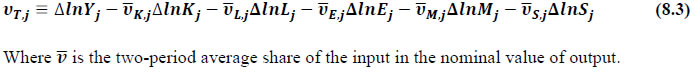 We define the value share of each input as: 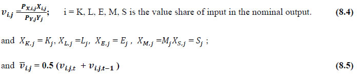 is the two-period average share for input Xi,j  Rearranging equation (8.3), yields the standard growth accounting decomposition of output growth into the contribution of each input and the TFP residual  where the contribution of an input is defined as the product of the input’s growth rate and its two period average value share. We can further decompose the contribution of each input into a quantity and quality component. As discussed earlier, the quality component represents substitution between H components, while the quantity component represents the increases in each detailed input. Our extended decomposition of the sources of output growth is given as follows:  Where Z is the stock of industry capital, Qk is the capital quality, H is number of persons employed and Ql is the quality of labour. The data series at individual industry level constructed for gross value added and gross output, labour input, capital input, intermediate inputs and factor income shares (described in Chapters 2, 3, 4, 5, 6 and 7 respectively) are used to estimate TFPG during the period 1980 to 2019. Labour input is measured by using total person worked along with the labour quality index (see Chapter 4 for a detailed discussion). The series on growth rate in capital services forms the measure of growth in capital input (discussed in Chapter 5). TFPG estimation is done by using the gross output function framework21 (i.e. equation 8.7). 8.2 Methodology for Aggregation across IndustriesWe also provide the TFPG for aggregate economy and two broad sectors, viz. manufacturing and services.22 However, the method of estimation of TFP growth for individual industries described in section 8.1 cannot be readily applied to a higher level of aggregation. The main problem is that gross value of output cannot be added across industries to generate a measure of output at a higher level of aggregation, say for the economy or of any of the broad sectors. Therefore, it becomes necessary to consider appropriate methods of aggregation across industries consistent with the gross output function specification of technology at the individual industry level. We use the Törnqvist index23 for aggregating across the broad sector and total economy. Taking this approach, computations are made for the manufacturing sector, the services sector, and for the aggregate economy. These aggregates are obtained using Tornqvist aggregate of growth rates of real value added, capital input, and labour input. Below, we briefly describe the Törnqvist index. Suppose the aggregate sector J consists of n KLEMS industries (j=1:n). We obtain the output (vale added) and inputs aggregates for sector J as: 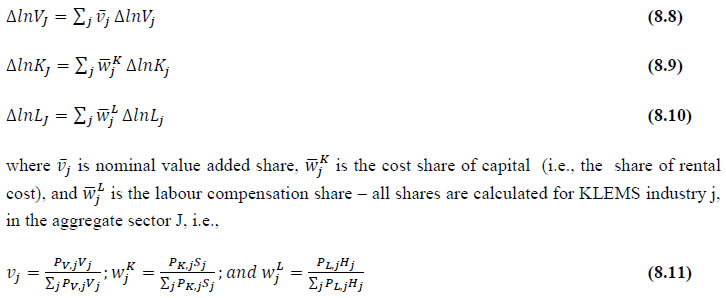 where PV,j is the price of value added in industry j, Vj is the real value added in industry j, PK,j is the rental price of capital in industry j, Sj is the capital stock in industry j, PL,j is the wage rate (price of labour) in industry j, and Hj is the employment in industry j. The aggregate output (real value added) and input growth rates obtained above are then used with the growth accounting equation to obtain the sectoral TFP growth rates. 1 From both aggregated 9 NAS sectors Gross Domestic Product by economic activity statement along with the disaggregated statements of these 9 NAS sectors. 2 In the EUS, the persons employed are classified on the basis of their activity status into usual principal status (UPS), usual principal and subsidiary status (UPSS), current weekly status (CWS) and current daily status (CDS) for quinquennial rounds. refer to Appendix A for detailed definition of UPSS, CWS and CDS. 3 This is also the mid-point of financial year 4 For more detailed discussion on extrapolation and interpolation of the series, readers may refer to KLMES data manual version 2020 released by RBI on its website 5 In PLFS, the earnings by self-employed are also provided, but for consistency with other rounds we have used the same procedure of Mincer equation even for this round. In EU KLEMS (Timmer, et.al., op cit; p 67) it is assumed that the earnings of the self-employed is equal to the earnings of ‘regular' employees. 6 For detailed explanation of Heckman two-step process one may refer to the previous year manual 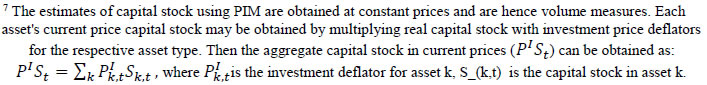 8 This version of the database does not make a distinction between ICT and non-ICT assets, as the industry level data on ICT assets are weak. An attempt to estimate aggregate economy level ICT capital can be found in Erumban and Das (2015). 9 See O’ Mahony and Timmer (2009) for a description of EU KLEMS database 10 This data is not publicly available. However, CSO has been kind to compile this data for the India-KLEMS project. 11 In some years transport equipment was provided as part of the machinery and equipment, categorized as ‘tools, transport equipment and other fixed assets. In such cases, we use transport/tools, transport and other fixed asset ratio in the nearest year to separate transport equipment. 12 A detailed discussion on how the series prior to 2011-2012 were adjusted to match the subsequent series is provided in Box 5.2A in the Appendix. 13 Gross investment is estimated as the difference between book value of asset in period t and in period t-1 and add depreciation in period t to that. 14 This choice is driven by the fact that the first year of availability of ASI data is 1964-65. 15 National Accounts Statistics-Sources and Methods, Chapter 26, CSO (2007), 16 We do not intend to delve into the controversies over the use of internal vs. external rate of return in the context of productivity measurement. This database uses See Erumban (2008a and b) for a discussion on these issues. 17 Reserve Bank of India, Handbook of Indian Statistics, Annual volumes. 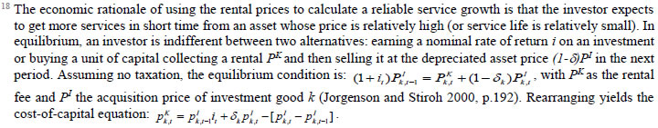 19 The estimation is done at group level rather than individual industries on the consideration that the group level estimates will be more reliable. 20 Consider, the semi-conductor (SC) industry, which is a key input to the computer hardware industry. Much of the output is invisible at the aggregate level because semi-conductor products are intermediate inputs to other industries rather than deliverables to final demand - consumption and investment goods. Moreover, SC plays a role in the improvements in quality and performance of other products like-computers, communication equipment and scientific instruments. Failure to account for them leads us to miss the role of key industries that produce intermediate inputs and importance of intermediate inputs for the industries that use them. (Jorgenson, Ho and Stiroh (2005), Productivity, volume 3). 21 It should be pointed out that an alternate set of estimates of TFPG obtained by using the value-added function framework is also provided in the India KLEMS dataset for which real gross value added is taken as the measure of output and only the two primary inputs are considered, namely labour input and capital input 22 More sophisticated methods of aggregation, such as the application of production possibility frontier approach or the application of direct aggregation is done in research papers written on the basis of the KLEMS dataset prepared. Such estimates of TFP growth are not a part of the database. 23 There exists other approaches to aggregate across broad sectors and industry, a detailed discussion on them can be found in KLEMS data manual version 2020 released by RBI on its website |
||||||||||||||||||||||||||||||||||||

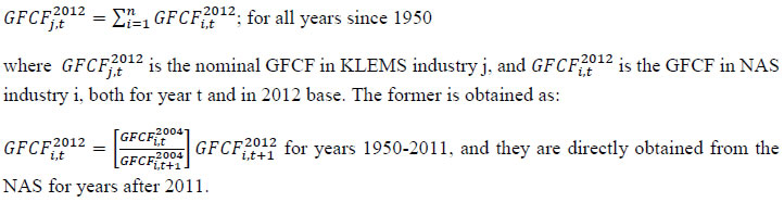
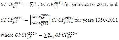
Measuring Productivity at the Industry Level – The India KLEMS Database
|
AUTHORS Sadhan Kumar Chattopadhyay Director Siddhartha Nath Assistant Adviser Sreerupa Sengupta Manager Shruti Joshi Manager
This document describes the procedures, methodologies and approaches used in the construction of India KLEMS database version 2023. The dataset includes measures of Gross Value Added (GVA), Gross Value of Output (GVO), Labour Employment (L), Labour Quality (LQ), Capital Stock (K), Capital Composition (KQ), the consumptions of Energy (E), Material (M) and Services (S) inputs, Labour Productivity (LP) and Total Factor Productivity (TFP). The database covers 27 industries comprising of the entire Indian economy. The database also provides these estimates at the broad sectoral levels (agriculture, manufacturing and services) and at the all-India levels. In the current version of the database covers the period from 1980-81 to 2021-22. The series have been constructed on the basis of data compiled from NSO, NSSO, ASI, Input-Output tables (I-O tables) and processed according to appropriate procedures. These procedures were developed to ensure harmonization of the basic data, and to generate growth accounts in a consistent and uniform way. Harmonization of the basic data has focused on several areas such as industrial classification, and aggregation levels. The production and publication of India KLEMS database are meant to support empirical research in the area of economic growth and its sources. Most importantly, the database is meant to support the conduct of policies aimed at supporting the acceleration of productivity growth in the Indian economy. The India KLEMS database, in this regard, provides a comprehensive measurement tool to monitor and evaluate productivity growth in Indian economy. Finally, the construction of the database would also support the systematic production of reliable statistics on growth and productivity using internationally comparable methodologies based on India’s national accounts, input-output tables and labour market surveys. The work relating to compilation of India KLEMS data was being done by the India KLEMS team housed at the Centre for Development Economics, Delhi School of Economics until the end of 2020. The work has been shifted to the KLEMS Division of Department of Economics and Policy Research of RBI since February 2021. The KLEMS Division at RBI compiled the India KLEMS data under the supervision of India KLEMS team until 2022. The current version of the India KLEMS Database, released hereby, is the second independent compilation of this data by the KLEMS Division in RBI, after the previous release of the data in 2023. 1.2 Coverage: Industries and Variables In this section we describe the coverage of India KLEMS database in terms of industries and variables. The database is created for 27 industries. The industrial classification is constructed by building concordance between NIC 2008, NIC 2004, NIC 1998, NIC 1987 and NIC 1970 to generate a uniform definition of ‘industries’ since 1980-81. This classification is very close to the International Standard Industrial Classification (ISIC) revision 3. The 27 industries are aggregated to form six broad sectors, namely:
Table 1.1 provides a listing of the 27 industries, including the higher aggregates. For detailed classification and concordance of study industries with NICs, readers may refer to Version 8 of the manual published in 2022. Table 1.2 provides an overview of all the series included in our database. Measures of Capital (K), Labour (L), Energy (E), Material (M) and Service (S) inputs as well as Gross Output (GO), have been constructed using National Accounts Statistics (NAS), Annual Survey of Industries (ASI), NSSO rounds and Input-Output (IO) Tables. In building annual time series on gross output, five inputs and factor income shares, various assumptions are made to fill up gaps in industry details and link series over time. As we know that NSSO rounds of unregistered manufacturing, Input Output Transaction Tables, and Employment and Unemployment Surveys by NSSO are available only for certain benchmark years., the use of information from these data sources necessitates interpolation and assumption of constant shares for building series of output and inputs. Further the construction of growth accounting series like total factor productivity, labour productivity, etc. are based on theoretical models of production and needs additional assumptions that are spelt out in subsequent chapters of the manual. Finally, the other Series like NDP at factor cost, compensation of employees, etc. are additional series which are used in generating the growth accounts and are informative by themselves. Chapter 2: Gross Value-Added Series at the Industry Level This chapter describes the data sources and methodology used to construct the Gross Value Added (GVA) series at current and constant prices for 27 study industries for the period of 1980-81 (1980) to 2021-22 (2021). The National Accounts Statistics (NAS) brought out by the NSO (National Statistics Office, Government of India) is the basic source of data for the construction of series on gross value added for INDIA KLEMS-industries. Up to 2011-12, estimates of GVA at both current and constant (2011-12) prices for all industries are obtained from Back Series of National Accounts (Base 2011-12). For years after 2011-12, they are directly obtained from NAS 2023. However, NAS estimates of value added are not available for a few India KLEMS industry groups. Therefore, we had to split some of the aggregate industry groups from NAS. Maintaining consistency with NAS, the value-added data in India KLEMS is measured at basic price. The construction of Gross valued added series involves three steps. Step 1: A concordance table between the classification used in the NAS and the 27 study industry classification used for this project has been prepared. Further, concordance between all the 27 sectors has been constructed with NIC- 1970, 1987, 1998, 2004 and 2008. Out of the 27 study industries, for 20 industries, GVA series both in current and constant prices is directly taken from NAS1. The sectors for which data are provided in NAS are Agriculture, Forestry & logging, Fishing, Mining and Quarrying, Manufacturing, Electricity,gas and water supply, Construction, Trade, Hotels & Restaurants, Railways, Transport by other means, Storage, Communication, Banking & insurance, Real estate, Ownership of Dwelling & Business Services, Public Administration & Defense and Other Services. Step 2: For manufacturing industries where direct estimates of GVA were not available from NAS, estimates have been made using additional information from ASI and NSSO unorganized manufacturing data. In these cases, GVA data is constructed by splitting the NAS data using ASI or NSSO distributions. ASI data (annual) has been used for registered and corporate manufacturing whereas interpolated ratios from NSSO 40th (1984-85), 45th (1989-90), 51st (1994-95), 56th (2000-01) 62nd (2005-06), 67th round (2010-11) and 73rd round (2015-16) rounds have been used for Unregistered and household manufacturing segments. For unregistered manufacturing for years 2015-16 to 2021-22 the ratio obtained from 73rd round of unregistered manufacturing has been used for the splitting. Table 2.1 and Table2.2 showcases the methodology used to split GVA of certain NAS sectors to match concordance with our classification. It is important to note that the industry-level value added volume indices are based on NAS. NSO provides single deflated value-added estimates for all sectors except Agriculture. Step 3: According to India KLEMS, GVA is adjusted for Financial Intermediation Services Indirectly Measured (FISIM). The detailed method of FISM adjustment is provided in earlier versions of the KLEMS manual. Chapter 3: Gross Output Series at the Industry Level This chapter describes the procedures and methodologies used in constructing the database for gross output series at the industry level over the period 1980-81(1980) to 2021-22(2021). To construct the gross output series at industry level, we use multiple data sources namely National Accounts Statistics, Annual Survey of Industries, NSSO rounds for unorganized manufacturing and Input Output Transaction tables. The data sources and methodology used are documented below: National Accounts Statistics: The NAS is the basic source of data for the construction of time series on the gross output. The NAS back series 2011 with base 2004-05 and NAS 2014 provides estimates of gross output for six disaggregate industries at current and constant prices since 1950-51 till 2011-12. These sectors are Agriculture, Mining and Quarrying, Construction and Manufacturing sectors (Registered and Unregistered Manufacturing). However, the Back Series with base 2011-12, which is the source of GVA in India KLEMS database 2022, does not provide estimates of GVO for most of the industries except for Agriculture, Mining and Quarrying and Construction. For these three industries, GVO data at current and constant were prices directly obtained from Back Series with base 2011-12. Therefore, for the 1980-81 to 2011-12 period, we estimate the GVO series for the remaining 24 industries at current and constant prices by applying the respective GVO/GVA ratio for current and constant prices obtained from Back Series with base 2004-05 and NAS 2014 to GVA with 2011-12 base. For years since 2011, we have taken the estimates of GVO both at current and constant prices for all industries directly from NAS 2023. (a) Filling procedures of National Accounts series: It is to be noted that the NAS estimates of gross output for a few industry groups are at a more aggregate level, requiring splitting of the aggregates. In such cases, NAS estimates of output have been split using additional information from the Annual Survey of Industries and NSSO rounds of Unregistered Manufacturing to obtain estimates at a higher level of disaggregation. Secondly, for Unregistered manufacturing gross output data is available in NAS from 2004-05 onwards. In this case, information from NSSO survey rounds has been used for missing years to derive output estimates of unregistered manufacturing industries at current and constant prices. As mentioned earlier, for the gross value-added series of service sectors we obtain our estimates from NAS. However, prior to 2011-12 National Accounts did not provide any estimates of the gross output of service sectors and hence we rely on Input output transaction tables ( from which the ratio of gross to value added is computed which is then applied to GVA reported in NAS) which are available at an interval of 5 years or so. This necessitates interpolation and assumption of constant shares for measuring output of services sectors. The Input Output Transaction Tables for Benchmark years of 1978-79, 1983-84, 1989-90, 1993-94, 1998-99, 2003-04 and 2007-08 are used to derive gross output series for service sectors. The construction of the gross output series at current and constant prices involves the following steps: Step 1: Measuring Gross Output of Agricultural Sector, Mining and Quarrying, and Construction NAS provides nominal and real GVO series for a) Crops and Plantation, b) Animal Husbandry c) Forestry and Logging d) Fishing. By aggregating the GVO of these four subsectors we derive the GVO of Agricultural sector. The Gross output estimates of Mining and Quarrying and Construction at current and constant prices from 1980-2022 is also directly taken from NAS. Step 2: Measuring Gross Output of Manufacturing Industries Since 2011-12, gross output data for 7 out of 13 manufacturing industries listed in table 3.1 are directly picked up from NAS. For the remaining 6 sectors output is constructed by splitting the NAS output data using ASI or NSSO distributions. ASI data (annual) has been used for registered manufacturing whereas interpolated ratios from 67th (2010-11) and 73rd (2015-16) rounds have been used for Unregistered Manufacturing segments. A list of study industries is presented in Table 3.2 showcasing the methodology used to split GVO of certain NAS sectors to match concordance with our classification for the year 2011 to 2022. Step 3: Measuring Gross Output for Services Sectors and Electricity, Gas and water supply Since 2011 -12 NAS provided estimates of GVO at current and constant prices. Prior to 2011-12 Gross Output series for Services sectors and sector Electricity, Gas and Water supply have been constructed using information from Input – Output Transaction Tables of the Indian economy published by CSO. The details method of construction of GVO back series for services is provided in earlier versions of KLEMS Data manual. Chapter 4: Labour Input Series at the Industry Level This chapter discusses the construction of labour input for 27 industries from 1980-81 to 2021-22. Labour input captures both the quantity of labour (i.e. number of persons) and quality of labour over time. Labour quality is measured based on educational qualification and wage rates of the workers within each of the 27 industries. Given the limitations of India’s employment statistics (Sivasubramonian; 2004, & Himanshu; 2011, Ghose; 2016), especially the availability of information on wages/ earnings of different category of workers across industries, the database provides only the labour quality index based on five different education categories. Labour input is measured by multiplying the number of persons employed by the index of labour quality which captures the human capital embodied in the labour, constructed separately for each industry. The 38th to 68th rounds of the Employment and Unemployment Survey (EUS) by India’s National Sample Survey Office (NSSO) conducted between 1983 and 2011-12, respectively, and the Periodic Labour Force Survey (PLFS) rounds of 2017-18, 2018-19, 2019-20,2020-21 and 2021-22 by National Statistical Organization (NSO) are the main sources data for estimating labour input. Additionally, for estimating India’s population growth rate, we used India’s decadal census and country-wise population growth rates by the World Bank. Methodology The total employment, measured by the number of persons engaged in each of the 27 industries in India is computed as follows: 1. First, the concordance between 27 KLEMS industries was built with each of NIC-1970, 1987, 1998 and 2008, separately. 2. Based on each round of EUS and PLFS, the distributions of workers by UPSS2 across the four components - Rural Male, Rural Female, Urban Male and Urban Female were obtained. These distributions of workers were then multiplied with the all-India figures for the number of workers for each of the years of EUS and PLFS rounds. 3. The all-India figures for the number of workers are generally not directly available from any official sources. We obtain the official estimates of worker-population ratios (WPR) from each of the survey rounds and multiply them with India’s total population for the survey year. We obtain India’s population for the survey years by interpolating India’s decadal census populations. 4. For 2017-18, 2018-19 and 2019-20, the all-India figures for number of employed persons were available from the Government of India. These figures were directly used in the estimates. 5. For 2021-22 and 2021-22, we had to project India’s total population. For this, we used the annual population growth rates for India provided by the World Bank. We scaled up the World Bank estimates with the same proportion by which India’s population growth rate in 2011-12 based on the latest Census Report exceeded that of World Bank estimates. 6. Finally, we obtain Lij for each industry where i=1 for rural and 2 for urban sectors, and j=1 for male and 2 for female for each round. 7. Total persons employed in a year were then obtained for each industry as the sum of the Lij over gender and sectors, i.e., ΣiΣjLij. 8. The estimates of employment for the intervening years between each of the EUS and PLFS rounds are obtained by simple interpolation across the four segments- rural male, rural females, urban male and the urban females for all of the 27 industries separately. 9. The mid-points of the surveys are around the mid-year of the survey rounds, i.e July for 38th round and 1st Jan for the other rounds; whereas the interpolation has been centered around 1st October which is the mid-year of the national income estimates3. Hence, the base is shifted to October of each year while interpolating4 the values. This is done to coincide the survey year mid-point to the mid-point of financial year. For extrapolation backward to 1980-81 to 1982-83, the interpolation of the broad industrial classifications of 32nd round (1977-78) and 38th round (1983-84) are used. Thus, the estimates from 32nd round are mainly used as control numbers. Between 2005 and 2011, we observed very high growth rate in number of employed persons series for the industry Electrical and Optical Equipment as compared to other manufacturing industries and the overall growth in employment in this industry during 2005-2011 was found to be higher than that for Construction (which seems somewhat unrealistic). It was also observed that there was a negative growth in employment in Textiles, Textile Products, Leather and Footwear although real GVA of this industry more than doubled between 2005 and 2011. To address these issues, some adjustments to the initial employment estimates for Electrical & Optical Equipment and Textiles, Textile Products, Leather and Footwear have been done. Onwards 2005, employment series for Electrical & Optical Equipment has been estimated applying annual growth rates obtained from ASI and NSSO rounds to the number of employed persons for the year 2005-06. Then, for the years 2005-06 to 2011-12, we compute the difference between estimated employment series from EUS rounds and that based on ASI & NSSO rounds for the Electrical and Optical Equipment industry and add it to Textiles, Textile Products, Leather and Footwear industry. This ensures that for the manufacturing as a whole our estimates remain the same as obtained from EUS rounds. 4.2 Estimation of Labour Quality index The quality of labour force is of considerable importance in the context of productivity measurement, and one of the widely used methodologies to capture changes in labour quality is given by Jorgenson, Gollop and Fraumeni (JGF) (1987). In growth accounting methodology of measurement of total factor productivity (TFP) when output growth is decomposed into growth of inputs and the residual TFP, then labour input is measured as an index of labour service flows. It accounts for changes in labour quality in terms of labour characteristics such as educational attainment, age (experience), gender, employment status, etc. and thus accounts for heterogeneity of the labour force. In our study, the index of aggregate labour quality measures the changes in the composition of labour in the economy. The present study has computed labour quality index by using only education characteristic in the JGF methodology. Thus, the data required for the labour quality index in the present case, is employment and earnings by education and by industry. The labour quality index has been computed using five education categories namely- up to primary, primary, middle, secondary & higher secondary, and above higher secondary. There are thus five types of persons employed for each of the 27 study industries. The quality growth rates are estimated for total persons employed in these industries in India for the 38th, 50th, 55th, 61st, 68th rounds of EUS by NSSO, and all the PLFS rounds upto 2021-22. They are then indexed to 1983-84 (38th round) as the base, so as to assess the temporal changes in labour’s skill. Interpolation has been done between the major rounds for values of the intermediate years. Since the series is required from 1980-81, we have extrapolated it backwards from 1983-84 and the index is recomputed with base 1980-81 equal to 100. The following steps have been performed: 1. Compute the distribution of persons employed by the five educational groups for all the 27 industries for the selected major rounds of EUS and PLFS. 2. Apply these proportions to the number of employed persons in different industries in the major rounds and PLFS to obtain the distribution of persons by education groups. 3. Estimate the earnings data from NSO which relates to mainly to the regular and casual persons employed. It may however be mentioned that even for these two groups, for a large number of persons employed, the wages are either missing or given as zero. For these employed persons whose wage information is missing, a Mincer equation is used to estimate the earnings for self-employed persons, using5 a Mincer wage equation, which is corrected for sample selection bias by using the Heckman’s6 two step procedure. The Mincer function has been applied to the earnings of casual and regular employees where the earnings have been regressed on the dummies of age, gender, education, location (rural or urban), marital status, social exclusion and industry. The corresponding earnings of the self-employed are obtained as the predicted value with similar traits. The average wages per day are then computed for persons employed of different type of employment, i.e., self-employed, regular and casual combined together; whose wages are available. 4. Based on steps 1 to 3, labour quality index is estimated as equation 4.1 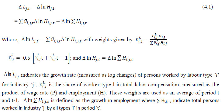 The first term of equation 4.1 indicates the changes in labour quality index, which is due to the changes in the composition of workers and the second term indicates the change in total persons employed in sector ‘j’. The index of aggregate labour quality thus measures the changes in the composition of labour in the economy The labour input (adjusted labour persons) then can be obtained by multiplying the number of persons employed by the corresponding labour quality index and the labour input growth is finally obtained by combining the growth of persons employed and the growth in the index of labour quality. Chapter 5: Capital Services Series at the Industry Level This chapter outlines the methodology employed to estimate capital Services for the 27 industries in India KLEMS database version 2023. All the productivity calculations in India KLEMS use capital services as an input to production, which is estimated using the approach developed by Jorgenson and Griliches (1967), and outlined in Jorgenson, Gollop, and Fraumeni (1987). The estimation of capital service growth rate is accomplished by first estimating capital stock for different assets, and then aggregating them across assets after correcting for the differences in their marginal productivities. Capital services account for the differences in marginal productivity between different asset types while capital stock measures only the vintages of capital, they do not account for asset heterogeneity. For instance, aggregate capital stock measures would assume that a computer's productivity is the same as that of a car. However, proper measures of capital stock would account for the decline in the efficiency of both computers and cars over their lifetime. Following an overview of the theoretical method to measure capital services (Jorgenson and Griliches,1967; JGF, 1987), the chapter discusses the specific empirical approaches we follow to implement these methods within the constraints of data availability for Indian industries. In India KLEMS, we have reported capital stock, capital services and the capital “capital composition effect”. Capital stock is reported in constant price volumes, and growth rates, while the latter two are reported in growth rates and indices. To measure capital services, using the Jorgenson and Griliches (1967) approach, we need estimates of capital stock for detailed asset types and the shares of each of these assets in total capital remuneration. The aggregate capital services growth rate is derived as a weighted growth rate of individual capital assets, the weights being the shares of each asset in the total compensation made to capital, i.e, 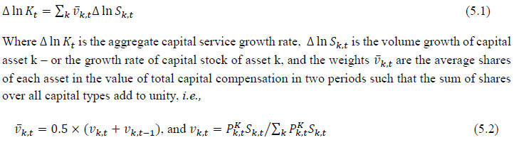 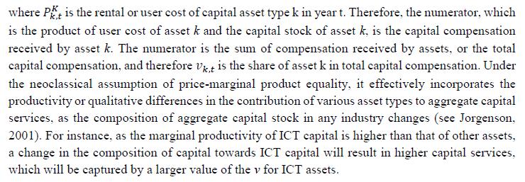 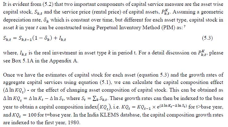 Since our measure of capital input takes account of asset heterogeneity, it was essential to obtain investment data by asset type. We distinguish between 3 different asset types – construction, transport equipment, and machinery (includes ICT and non-ICT machinery).8 We exploit multiple sources of information for the construction of our database on capital services. This includes the National Accounts Statistics (NAS) that provide information on broad sectors of the economy, the Annual Survey of Industries (ASI) covering the organized manufacturing sector, the National Sample Survey Office (NSSO) rounds for unorganized manufacturing and various Input-Output tables. Even though we use multiple sources of data, our final estimates are fully consistent with the aggregate data obtained from the NAS. In addition, our approach to capital measurement is consistent with international practices such as the EU KLEMS9, which ensures the possibility of international comparisons. In what follows, we discuss the various sources of data for asset wise investment and the construction of the relevant variables, in detail. (a) Asset-wise investment for broad sectors of the economy Industry-level estimates of capital input require detailed asset-by-industry investment matrices. NAS provides information on aggregate capital formation by industry of use for nine broad sectors, which, nevertheless, was not sufficient for our purpose. Therefore, we have collected more detailed data on assets and industries from the CSO.10 This is the data underlying the published aggregate gross fixed capital formation by the broad industry groups, separately for public and private sectors. For those sectors for which the investment matrices were not available from CSO, we gather information from other sources (e.g. ASI for organized manufacturing and NSSO surveys for unorganized manufacturing) and benchmark it to the aggregate investment series from the National Accounts. The data used in the current version of the India KLEMS is based on the revised NAS with 2011-2012 base and is available only since 2012. Therefore, for earlier years, we extrapolate the series using growth rates from previous version of the data. Table 5.1 provides an overview of asset types available in NAS and their corresponding asset types used in our study. Investment in education and health are obtained directly from national accounts for the period after 2012, for each asset. For years before 2012, we assume the trend in the distribution of output, in order to split the total investment in the aggregates of these sectors into sub-sectors.
Total investment in each asset category is calculated as the sum of private and public sector investment in each asset. Investment in transport equipment was not available separately for the private sector industries. Therefore, we distributed the NAS total machinery in the private sector using the industry distribution of machinery and transport equipment. These estimates are then subtracted from each industry’s total machinery & transport equipment data to obtain the transport equipment investment in the private sector industries. Using this approach, we could generate investment in transport equipment by industries for the period 1950-2016. We assumed the share of transport equipment in the total machinery and equipment group in 2016-2017 to remain to remain unchanged in subsequent years while estimating nominal investment in transport equipment in the similar way. The nominal investment was deflated using GFCF deflator for transport equipment (see section (c)). Since the distinction between registered and unregistered manufacturing is not available in the NAS since 2016, we used a quick fix to split these two. NAS provides a division between the corporate sector, public sector, and household sector. In the current version of the data, we consider the household sector as a proxy for unregistered and the corporate and public sector as a proxy for the registered sector. As mentioned earlier, the updates for years since 2017-2018 are solely based on published aggregate GFCF data from the National Accounts. In the 2019 version of the India KLEMS, we considered the 2012-2016 detailed asset-wise data by industries provided by the CSO as such and extended the data for 2017-2018 using the published aggregates. However, in the 2020 version of the data, we changed this approach, as there were some discrepancies between the published NAS totals and the detailed asset-industry data. While extending the past series of detailed asset-wise investments forward for years since 2017-2018 using the NAS-published headline series, we now consider the published NAS series as the benchmark since 2012. Then we apply the industry distribution of the 2012-2016 detailed series obtained previously from the CSO. The current approach is more appropriate and ensures a complete consistency with the NAS-published series. However, it may cause some changes in the capital service growth rates compared to the last release12. (b) Asset-wise investment for non-NAS sectors NAS provides data only for 9 broad sectors, while we have 27 industries, which necessitated further splitting of some of the NAS sectors. This includes aggregate manufacturing (registered and unregistered separately for the period 1950-2016) with 13 sub sectors; other services into 4 sub sectors; and real estate activities and business services into 2 sub sectors. The manufacturing sector investment data was disaggregated into 13 subsectors at the 2-digit level of NIC 1998 using ASI and NSSO data, which will be discussed in detail subsequently. Investment series in service sector has been split into sub sectors using two alternative approaches–value added shares, and capital/labour ratio in the higher aggregate industry. However, the final data used are based on value added shares, as we did not see any significant difference between the two. Registered (organized) Manufacturing: In order to split the aggregate capital formation in organized manufacturing sector into 13 study sectors, we use the ASI. ASI defines GFCF as actual additions (newly purchased, second hand and own construction) minus deductions plus depreciation adjustment for discarded assets during the year. This approach is based on a single year’s sample and helps to avoid potential huge negative investment series, and is also consistent with published ASI GFCF series. The yearly detailed volumes beginning 1964-65 were used to derive the gross fixed capital formation by asset type directly. For the years 1964-1978, the relevant data are obtained from published detailed volumes. For the period, 1983-84 to 2004-05 ASI has generated detailed tables from Block C of ASI schedule that contain data on fixed assets. Data for missing years are interpolated using the changes in investment using book value method13. Table 5.2 provides an overview of the asset categories available in ASI, and the relevant asset categories in our study to which they are attributed. Though ASI provides investment in land, for reasons of NAS consistency we exclude it from our database. Once investment in each of these assets and industries are generated using ASI data, we apply this industry-asset distribution to the published aggregate NAS GFCF series for organized manufacturing sector. It may also be noted that from 1960-61 to 1971-72, ASI data are for the census sector and from 1973-74 onwards they are for the factory sector. In order to make these two series comparable over years, we convert the data prior to 1972 to factory sector using the factory/census ratio in 1973. Thus, after these adjustments, we obtain investment data for 13 manufacturing sectors, by asset types, consistent with the NAS aggregate for registered manufacturing. This approach was accurate for the period 1950-2016 when the NAS provided aggregate registered manufacturing GFCF data. For the years after 2016, since when NAS does not provide registered manufacturing aggregate, we proxy registered manufacturing by the sum of public sector and corporate sector. Unregistered (unorganized) Manufacturing: The data required for creating the gross investment series for the 13 sectors of the unorganized manufacturing sector are obtained from various rounds of NSSO surveys on unorganized manufacturing. We use 6 rounds of NSSO surveys that cover the period 1989-2016. These are 45th round (1989-90), 51st round (1994-94), 56th round (2000-01), 62nd round (2005-06), 67th round (2010-11) and 73rd round (2015-16). Unit level data has been aggregated to 13 industries using the appropriate concordance. NSSO provides net addition to owned assets during the reference year within the block of fixed assets, and we use this as a measure of our investment. The investment series arrived at for six rounds were interpolated to obtain the annual time series of unorganized gross fixed capital formation by asset type. As in the case of registered sector, once the investment by asset types across industries are constructed, the asset-industry distribution is applied to the published NAS aggregate GFCF in unregistered manufacturing to obtain NAS consistent GFCF by asset type and industries. (c) Investment Prices by Asset Types In order to compute asset wise capital stock using PIM (equation 5.3) and rental price (see Box 5.1A in the Appendix), we require asset wise investment price deflators. Since CSO has provided us with investment data by industries and assets both in current and constant prices, we could derive the price deflators with base 2011-2012. For years before 2011, prices were spliced using 2004-2005 base investment deflators. These deflators are directly used for all the three asset categories we have. Since there was no separate asset wise data available for transport equipment in 2017-2018, the investment deflator for transport equipment from 2016-2017 was extrapolated using the trend in the investment price of total machinery & equipment, obtained from NAS. (d) Initial Stock, Depreciation Rates and Rate of Return For the implementation of PIM to estimate asset wise capital stock, we require an estimate of initial benchmark stock (see Erumban, 2008b for an in-depth discussion on this issue). NAS provides estimates of net capital stock since 1950 for all the broad sectors in its Statement 17: Net Fixed Capital Stock by industry of use. We take the NAS estimate of real net capital stock in 1950 (in 1999-2000 prices) as our benchmark stock for all non-manufacturing sectors, and for manufacturing sectors the same is taken for the year 1964.14 However, since the NAS estimate is available only for broad sectors and for aggregate capital, we use our industry-asset distribution of GFCF in order to create net fixed capital stock estimates by asset type for all the 27 sectors. The approach to split asset-wise capital stock is changed in the 2020 version of the India KLEMS database. Instead of using the GFCF distribution, we use the distribution of net capital stock by assets, available from the detailed asset data obtained from the CSO. Since the initial stock depreciates over the years, the impact of this change in distribution on the capital stock will vanish over the years at the individual asset level. However, as it changes the distribution of assets in the total capital stock, these compositional changes tend to have a visible impact on the aggregate capital stock, causing a historical revision of capital stock growth rates in some industries (esp. transport and storage, education, hotels and restaurants, electricity, transport equipment, etc.). NAS also provides detailed tables on assumed life of assets used for computing capital stock, for private units, administrative units as well as departmental and non-departmental units by asset types.15 We use these estimates of lifetime to derive appropriate depreciation rates for non-ICT assets, using a double declining balance rate. Following the NAS, we assume 80 years of lifetime for buildings, 20 years for transport equipment, and 25 years for machinery and equipment (see Appendix 26.2; CSO, 2007). The final depreciation rates used in the study are given in Table 5.3 by asset type. Subsequently, we build our capital stock series by asset types for all the 27 industries using our GFCF series from 1950 (1964) onwards for the non-manufacturing (manufacturing) sectors. Our measure of capital input is arrived using equation (5.1), for which we also require estimates of rental prices (see Box 5.1A in the Appendix). Assuming that the flow of capital services is proportional to the capital stock at individual asset level, aggregate capital flows can be obtained using a translog quantity index by weighting growth in the stock of each asset by the average shares of each asset in the value of capital compensation, as in (5.1). The rate of return (i) in equation (5.4) represents the opportunity cost of capital, and can be measured either as internal (or ex post) rate of return, or as an external (ex ante) rate of return. 16 The present version of the database uses an external rate of return, proxied by average of return on government securities and prime lending rate obtained from the Reserve Bank of India 17. Therefore, we use a real rate, which is net of capital gain. Hence, the capital gain component in equation is excluded while estimating rental price using external rate of return, obtaining  Where r is the real rate of return, nominal interest rate adjusted for consumer price inflation rate. The consumer price indices (CPI) are obtained from IMF and World Bank. The measures of capital input available in India KLEMS are based on only three asset categories, construction, machinery, and transport equipment. Therefore, it does not consider the enormous and distinct role of ICT capital in contributing to productivity and growth. The absence of ICT estimates in the database is driven by insufficient data on investment in ICT assets, such as hardware, software, and communication equipment in the National Accounts. However, during recent years, NAS has extended its asset coverage to include software and ICT equipment. Erumban and Das (2016) have made some estimates for the aggregate economy using input-output tables for ICT equipment and relying on NAS for software investment. Similarly, Erumban and Das (2020) have made some initial estimates of ICT capital by industries, which still remains a challenging task. Nevertheless, now that more data is available from NAS, it is possible to explore this further, and future extensions of the database may explore this. Similarly, following the SNA 2008 guidelines, the NAS now provides estimates of intangible capital such as intellectual property and research and development (R&D), which may be a useful extension to the capital input database. Two additional challenges are arising since the new system of national accounts. The first is the lack of separate data on registered and unregistered manufacturing, which poses challenges in using ASI and NSSO data to split aggregate manufacturing data into 13 industry groups. Instead of the registered and unregistered split, CSO now provides a division between the household and corporate sectors. We currently address this challenge by considering the household sector as unregistered manufacturing and the sum of public and corporate sectors as a registered sector. The second challenge is the lack of separate data on transport equipment and machinery assets in the new series of national accounts, which follows United Nation's System of National Accounts (SNA)-2008. Although, for the time being, we adopt ad-hoc approaches to fix this, it cannot be adopted on a long-term basis, which might necessitate combining transport equipment and machinery to one single asset. Finally, as mentioned earlier, the debate on whether it is appropriate to use an external rate of return or an internal rate of return is unsettled in the literature. It may be worth exploring estimates of capital using the internal rate of return. Appendix A: Some Discussions on the Estimation of Capital Services
Chapter 6: Intermediate Input Series at the Industry Level In this section, we describe the basic approach we have used to derive the volume series of Intermediate Inputs namely –Energy input (E), Material input (M) and Services input (S). The methodology for measuring industry output, intermediate inputs and value added was developed by Jorgenson, Gallop and Fraumeni (1987) and extended by Jorgenson (1990 a). The cornerstone of this approach is a time series of input output (IO) tables which gives the flows of all commodities in the economy, as well as payments to primary factors. Following a similar approach as explained in Jorgenson et al. (2005, Chapter 4) and Timmer et al. (2010, Chapter 3), the time series on intermediate inputs for the India KLEMS project have been constructed. Definition of EMS: As in EU KLEMS, this study identifies three main categories of Intermediate inputs. They are classified as follows: 1. Energy Input 2. Material Input 3. Service Input The following five energy types (and products) have been classified as the Energy input: 1. Coal and Lignite 2. Petroleum products 3. Electricity; (for electricity used in the electricity sector, since there is a good amount of inter-firm sale and purchase of electricity, it has been treated as material rather than as energy) 4. Natural gas 5. Gas (LPG) The following fourteen input items have been classified as the Service input: 1. Water supply 2. Railway transport services 3. Other transport services 4. Storage and warehousing 5. Communication 6. Trade 7. Hotels and restaurants 8. Banking 9. Insurance 10. Ownership of dwellings 11. Education and research 12. Medical and health 13. Other services 14. Public administration All other intermediate inputs barring the above mentioned nineteen inputs are classified as material input. The methodology for computation of Intermediate Input Series for 27 Industries from 1980-2022 at current and constant prices is explained in steps. Step 1: Concordance is done between IOTT and study industries
Step 2: Obtaining estimates for Material, Energy and Service Inputs for 27 Industries, in benchmark years
Thus, for each of the benchmark year, estimates are obtained for Material, Energy and Service Inputs that has been used to produce Gross output in the 27 different India KLEMS Industries. Step 3: Projecting a time series (1980 to 2019) of proportions of Material, Energy and Service Inputs in Total Intermediate Inputs for each of the 27 industries
There exists some abnormal fluctuation in the proportions of Material Inputs, Energy Inputs, and Service Inputs in Total Intermediate Inputs for benchmark years. In that case, we drop that specific benchmark proportion and linearly interpolate of the adjacent benchmark proportions to estimate proportion for intervening years. For the industry ‘Wood & Wood Products’, we estimated proportions of Material Inputs, Energy Inputs, and Service Inputs in Total Intermediate Inputs from SUT 2015-16 instead of Input Output Transaction Table 2015-16. For the industry group ‘Coke, Refined Petroleum and Nuclear Fuel’, we estimated proportions of Material Inputs, Energy Inputs, and Service Inputs in Total Intermediate Inputs from ASI data instead of Input Output Transaction Table. This has been done because the relevant proportions differed significantly between the input-out tables and ASI, and the latter is believed to be making a more correct assessment of energy inputs used in the Coke and Petroleum products industry. Step 4: Consistency with NAS The projection of intermediate input vector, using IOTT in Step 3 needs to be consistent with the estimated output from NAS.
1. For Benchmark years: Ratio of Total Intermediate inputs from NAS to that from IOTT is adjusted proportionately to the absolute value of Energy Inputs/Material Inputs/Service Inputs obtained from IOTT. 2. For Intervening Years: The interpolated proportions of Energy Inputs, Material Inputs and Services Inputs obtained from IOTT, is applied directly to the total intermediate inputs from NAS to get each inputs share. Steps 1-4: This gives a time series of Material, Energy, and Service Inputs for 27 study Industries from 1980 to 2022 at current prices. Steps 5 and 6 below, explain the methodology for computation of Intermediate Input Series for 27 study Industries from 1980 to 2022 at constant price. The approach followed here is to first form the aggregates of materials, energy and services at current price for each study industry from the benchmark Input Output tables and then develop deflators of Materials, Energy and Service Inputs for each of the 27 study Industries separately. Step 5: Constructing Deflators of Materials, Energy and Service Inputs for 27 study Industries separately
Step 6: Computing Time Series on Intermediate Input for 27 study Industries from 1980-2022, Constant prices
Thus, we have a time series of Material, Energy and Service Inputs for 27 study Industries at constant prices. Chapter 7: Factor Income Share Series at the Industry Level The distribution of income between capital, labour and intermediate inputs, is an important element in growth accounting because income shares, under conditions of competitive markets, can be used to measure the contributions each factor makes towards output growth. 7.1 Methodology for Measuring Labour Income Share Series Under the assumption of constant returns to scale with two factors of production i.e., labour and capital, the sum of the labour income share and capital income share is 1. The labour income share is defined as the ratio of labour income to GVA. Capital income share is accordingly obtained as one minus labour income share. There are no published data on factor income shares in Indian economy at a detailed disaggregate level. National Accounts Statistics (NAS) of the CSO publishes the NDP series comprising of compensation of employees (CE), operating surplus (OS) and mixed income (MI) for the NAS industries. The income of the self-employed persons, i.e., mixed income (MI) is not separated into the labour component and capital component of the income. Therefore, to compute the labour income share out of value added, one has to take the sum of the compensation of employees and that part of the mixed income which are wages for labour. The computation of labour income share for the 27 study industries involves two steps. First, estimates of CE and MI have to be obtained for each of the 27 study industries from the NAS data which are available only for the NAS sectors (see Table 7.1). Second, the estimate of mixed income has to be split into labour income and capital income for each industry for each year (except for those industries for which the reported mixed income is zero, for instance, public administration). Basis data sources used for the computation of labour income share are NAS, ASI and unit level data of survey of unorganized manufacturing enterprises. These data sources are used to obtain estimates of CE, OS and MI for each of the 27 study industries. For splitting the labour and non-labour components out of the mixed income of self-employed, the unit level data of NSS employment-unemployment survey are used along with the estimates of CE, OS and MI basically obtained from the NAS. a) Construction of Labour Income Share Series in Gross Value Added The estimation of labour income share for the 27 study industries has been done in two steps, as discussed below. Step 1: Estimation of CE, OS and MI for the 27 study Industries NAS provides estimates of compensation of employees (CE), operating surplus (OS) and mixed income (MI) for the 9 NAS industries in different annual Sequence of National Accounts reports. For some industries under study, for instance (i) Agriculture, forestry & logging and fishing, (ii) Mining & Quarrying, (iii) Electricity, gas and water supply and (iv) Construction, the required data are readily available from NAS. For others, the estimates available in NAS have to be distributed across the study industries using ASI data. The NAS estimates of factor incomes (CE) for registered manufacturing is split into KLMES 13 industries (3-15) in proportion to the reported ASI data on emoluments for various industries. Estimate of factor incomes for ‘other services’ in NAS has been split into estimates for (i) Education, (ii) Health and Social Work, and (iii) Other Community, Social and Personal Services including Renting of Machinery and Business Services, and Private Household with Employed Persons. Before 2011-12, NAS provides estimates of factor incomes for registered manufacturing and unregistered manufacturing, but not for individual manufacturing industries. However, 2011-12 onwards NAS disaggregated the manufacturing sector in corporate sector and household sector. The NAS estimates of factor incomes for registered manufacturing and corporate sector have to be split into various manufacturing industries considered in the study (13 in number) using ASI data. The reported CE in NAS for registered manufacturing and corporate sector has been distributed into those 13 industries in proportion to the reported ASI data on emoluments for various industries. In a similar way, using ASI data, the estimate of OS for registered manufacturing and corporate sector has been distributed. Emoluments are subtracted from gross value added for various industries yielding capital income. The share of different industries in aggregate capital income of organized manufacturing indicated by the ASI data is used to split the estimate of OS for registered manufacturing and corporate sector reported in the NAS. The methodology applied for unregistered manufacturing and household sector is similar. The published results and unit level data of survey of unorganized manufacturing industries have been used for this purpose. The estimates of wage payments (to hired workers) in different industries have been used to split (proportionately) the estimate of CE in the NAS for aggregate unregistered manufacturing. The estimated wage payment is subtracted from the estimated value added to obtain an estimate of capital income and mixed income of the self-employed in various unorganized manufacturing industries. The estimate of MI provided in NAS for unregistered manufacturing and household sector has then been proportionately distributed across industries using the estimate of capital income and mixed income of the self-employed in various industries that could be formed on the basis of published results and unit level data of survey of unorganized manufacturing industries. Unlike the ASI data for organized manufacturing, the data for unorganized manufacturing enterprises are available for only select years. The proportions mentioned above could therefore be computed only for those select years (data for six rounds have been used; these are for 45th Round (1989-90), 51st Round (1994-95), 56th Round (2000-01), 62nd Round (2005-06), 67th round (2010-11) and 73rd Round (2015-16)). It has accordingly, been necessary to resort to interpolation/extrapolation to obtain the relevant proportions for other years. Step 2: Splitting of MI into Labour Income and Capital Income As explained above, the income share of labour is computed as: 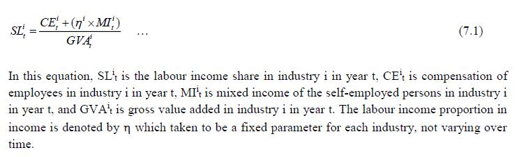 The derivation of the GVA series for different industries has been briefly explained in Chapter 2. The derivation of CE and MI series has been explained in step I above. Therefore, only the estimation method of η needs to be described. The estimation of η has been done with the help of NSS survey-based estimates of employment of different categories of workers (number of persons and days of work) and wage rates (which has been described briefly in chapter 4) coupled with estimates of MI, basically obtained from the NAS. Two approaches have been taken to get an estimate of η, and the labour income share series for different industries finally adopted in the study makes use of an average of the estimates of η obtained by the two approaches. In the first approach, an estimate of labour income of self-employed workers has been made for each study industry for eight years, 1983-84, 1987-88, 1993-94, 1999-00, 2004-05, 2009-10, 2011-12 and 2015-16 on the basis of the estimated number of self-employed, wage rate of self-employed and the number of days of work per week. The industry-wise estimates of number of self-employed, wage rate of self-employed and the number of days of work per week have been made from unit records of NSS employment-unemployment survey (major rounds) of 1983, 1993-94, 1999-00, 2004-05, 2011-12, and PLFS of 2018-19, 2019-20. 2020-21 and 2021-22. The estimates of the number of self-employed, wage rate of self-employed and the number of days of work per week provide an estimate of the annul labour income of self-employed workers which is divided by the mixed income of self-employed (derived from NAS) to get an estimate of η. For five industries, the ratio in question has been computed and applied. For the other 22 industries, the ratio in question has been computed after clubbing the industries into 11 industry groups.19 In the latter case, a common ratio computed for group of industries has then been applied to constituent industries. The list of industries or industry groups for which η has been estimated is given in table 7.2. In the second approach, the NSS data are used to compute the following ratio: the ratio of labour income of self-employed workers to the labour income of regular and casual workers. Let this be denoted by θ. Then, the estimate of CE provided in the NAS is multiplied by θ to obtain an estimate of the labour income component out of the MI reported in the NAS. The labour component of MI divided by total MI gives an estimate of η. In case the estimated labour component of MI exceeds the estimate of MI, the estimate of η has been taken as unity. Examining the estimates obtained by the first approach, it was found that the estimated labour income share out of mixed income varied significantly among the estimates for the seven years for which the ratio in question has been estimated. The estimates of η obtained by the second approach has the problem that in a number of cases, the estimated labour component of MI exceeds the estimate of MI given in the NAS, and therefore η is taken as one. The method finally adopted is as follows: (a) The average value of η has been computed for each industry or industry group by taking the estimates for the years 1983-84, 1987-88, 1993-94, 1999-00, 2004-05, 2009-10, 2011-12 and 2015-16. This has been done separately for the estimates based on approach-1 and those based on approach-2. (b) The estimates of η obtained for each industry or industry group by the two approaches have then been averaged. (c) Having obtained an estimate of η, equation 7.1 given above has been applied to compute the labour income share. b) Construction of Factor Income Share Series in Gross output The income share of labour, capital and intermediate inputs in Gross output has been computed using the following steps:
The splitting of unorganized sector factor incomes into individual industries has been done using unorganized survey results. The proportions computed for 1983-84 has been applied for the period 1980-81 to 1983-84. While there were surveys of unorganized manufacturing enterprises in 1978-79 the survey results have not been used for estimation of factor incomes in different industries of the unorganized manufacturing sector. Chapter 8: Growth Accounting Methodology This chapter deals with the methodology of measurement of total factor productivity (TFP) growth for individual industries in the KLEMS framework and the aggregation from industry level productivity measures to measures for broad sectors and the economy as a whole. The methodology of analysis of sources of gross output growth at the individual industry level and sources of GVA (Gross Value Added) or GDP growth at the broad sector level and economy level will also be presented in this chapter 8.1 Methodology for Measuring Productivity Growth at the Industry level The production function Our measurement of TFP growth for different industries of the Indian economy is based on a gross output production function for each industry j: Y = f(L(L1,…Ln), K(K1…Km), E(E1….Es), M(M1 …Mu), S(S1 … Sv), T) (8.1) Y is industry gross output, L is labour input, K is capital input and E, M and S are intermediate inputs-namely energy, material and services and T is an indicator of technology for industry j. All variables are indexed by time (t subscript is suppressed). There are several things to note about the production function - (1) all variables are aggregates of many components that have been discussed in the earlier report/chapters; (2) we assume that the industry production function is separable in these aggregates; (3) time (indicator of technology) enters the production function symmetrically and directly with inputs. An important feature of the gross output approach is the explicit role of intermediate inputs. In our study, we have considered three intermediate inputs - energy, material and services and this is important as we may find that intermediate inputs are the primary component of some industries outputs20. Failure to quantify intermediate inputs leads us to miss both the role of key industries that produce intermediate inputs and the importance of intermediate inputs for the industries that use them. To estimate the contributions of total factor productivity, and inputs to industry level output growth, based on the above-mentioned production function, we construct real values of inputs and output, using industry level price data for capital, labour and intermediate inputs, and output. e.g., PYj; PLj, PKj; PEj. PMj, PSj. The industry price of an input varies across industries due to compositional effects as industries expend different shares of their investment on each type of asset. The same is true for all inputs. Total Factor Productivity 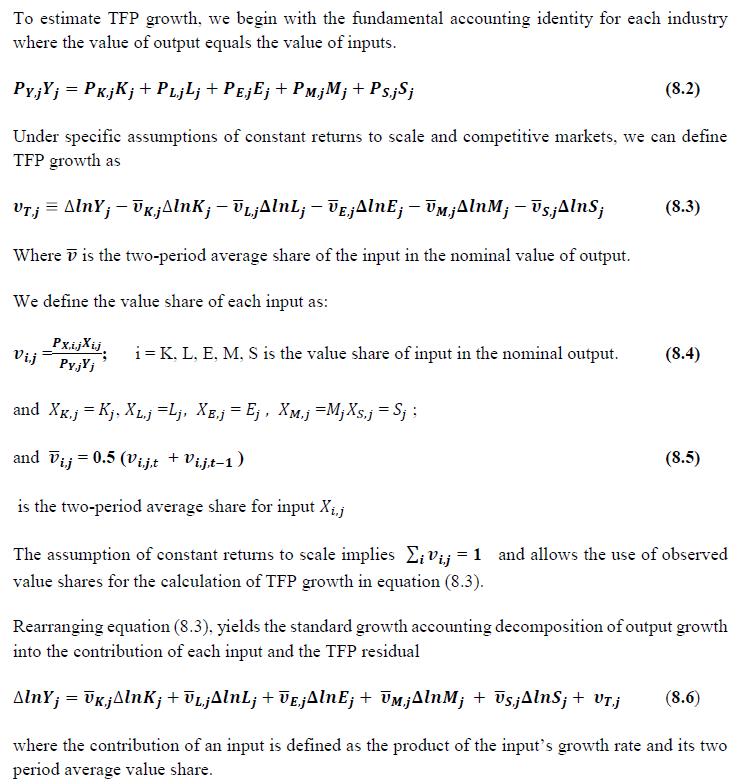 We can further decompose the contribution of each input into a quantity and quality component. As discussed earlier, the quality component represents substitution between H components, while the quantity component represents the increases in each detailed input. Our extended decomposition of the sources of output growth is given as follows:  Where Z is the stock of industry capital, Qk is the capital quality, H is number of persons employed and Ql is the quality of labour. The data series at individual industry level constructed for gross value added and gross output, labour input, capital input, intermediate inputs and factor income shares (described in Chapters 2, 3, 4, 5, 6 and 7 respectively) are used to estimate TFPG during the period 1980 to 2019. Labour input is measured by using total person worked along with the labour quality index (see Chapter 4 for a detailed discussion). The series on growth rate in capital services forms the measure of growth in capital input (discussed in Chapter 5). TFPG estimation is done by using the gross output function framework21 (i.e. equation 8.7). 8.2 Methodology for Aggregation across Industries We also provide the TFPG for aggregate economy and two broad sectors, viz. manufacturing and services.22 However, the method of estimation of TFP growth for individual industries described in section 8.1 cannot be readily applied to a higher level of aggregation. The main problem is that gross value of output cannot be added across industries to generate a measure of output at a higher level of aggregation, say for the economy or of any of the broad sectors. Therefore, it becomes necessary to consider appropriate methods of aggregation across industries consistent with the gross output function specification of technology at the individual industry level. We use the Törnqvist index23 for aggregating across the broad sector and total economy. Taking this approach, computations are made for the manufacturing sector, the services sector, and for the aggregate economy. These aggregates are obtained using Tornqvist aggregate of growth rates of real value added, capital input, and labour input. Below, we briefly describe the Törnqvist index. 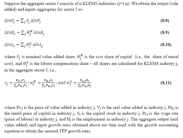 1 From both aggregated 9 NAS sectors Gross Domestic Product by economic activity statement along with the disaggregated statements of these 9 NAS sectors. 2 In the EUS, the persons employed are classified on the basis of their activity status into usual principal status (UPS), usual principal and subsidiary status (UPSS), current weekly status (CWS) and current daily status (CDS) for quinquennial rounds. UPSS refers to a person’s employment status based on what he/she might have been engaged in over a period of 365 days preceding the date of survey. 3 This is also the mid-point of financial year 4 For more detailed discussion on extrapolation and interpolation of the series, readers may refer to KLMES data manual version 2020 released by RBI on its website 5 In PLFS, the earnings by self-employed are also provided, but for consistency with other rounds we have used the same procedure of Mincer equation even for this round. In EU KLEMS (Timmer, et.al., op cit; p 67) it is assumed that the earnings of the self-employed is equal to the earnings of ‘regular' employees. 6 For detailed explanation of Heckman two-step process one may refer to the previous year manual 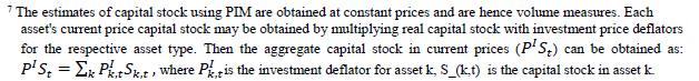 8 This version of the database does not make a distinction between ICT and non-ICT assets, as the industry level data on ICT assets are weak. An attempt to estimate aggregate economy level ICT capital can be found in Erumban and Das (2015). 9 See O’ Mahony and Timmer (2009) for a description of EU KLEMS database 10 This data is not publicly available. However, CSO has been kind to compile this data for the India-KLEMS project. 11 In some years transport equipment was provided as part of the machinery and equipment, categorized as ‘tools, transport equipment and other fixed assets. In such cases, we use transport/tools, transport and other fixed asset ratio in the nearest year to separate transport equipment. 12 A detailed discussion on how the series prior to 2011-2012 were adjusted to match the subsequent series is provided in Box 5.2A in the Appendix. 13 Gross investment is estimated as the difference between book value of asset in period t and in period t-1 and add depreciation in period t to that. 14 This choice is driven by the fact that the first year of availability of ASI data is 1964-65. 15 National Accounts Statistics-Sources and Methods, Chapter 26, CSO (2007), 16 We do not intend to delve into the controversies over the use of internal vs. external rate of return in the context of productivity measurement. This database uses See Erumban (2008a and b) for a discussion on these issues. 17 Reserve Bank of India, Handbook of Indian Statistics, Annual volumes. 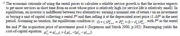 19 The estimation is done at group level rather than individual industries on the consideration that the group level estimates will be more reliable. 20 Consider, the semi-conductor (SC) industry, which is a key input to the computer hardware industry. Much of the output is invisible at the aggregate level because semi-conductor products are intermediate inputs to other industries rather than deliverables to final demand - consumption and investment goods. Moreover, SC plays a role in the improvements in quality and performance of other products like-computers, communication equipment and scientific instruments. Failure to account for them leads us to miss the role of key industries that produce intermediate inputs and importance of intermediate inputs for the industries that use them. (Jorgenson, Ho and Stiroh (2005), Productivity, volume 3). 21 It should be pointed out that an alternate set of estimates of TFPG obtained by using the value-added function framework is also provided in the India KLEMS dataset for which real gross value added is taken as the measure of output and only the two primary inputs are considered, namely labour input and capital input 22 More sophisticated methods of aggregation, such as the application of production possibility frontier approach or the application of direct aggregation is done in research papers written on the basis of the KLEMS dataset prepared. Such estimates of TFP growth are not a part of the database. 23 There exists other approaches to aggregate across broad sectors and industry, a detailed discussion on them can be found in KLEMS data manual version 2020 released by RBI on its website |
||||||||||||||||||||||||||||||||||||


భారతీయ రిజర్వ్ బ్యాంక్ మొబైల్ అప్లికేషన్ను ఇన్స్టాల్ చేయండి మరియు తాజా వార్తలకు త్వరిత యాక్సెస్ పొందండి!
మా యాప్ను ఇన్స్టాల్ చేయడానికి QR కోడ్ను స్కాన్ చేయండి


