 IST,
IST,
Chapter V: Open Economy Flexible Inflation Targeting
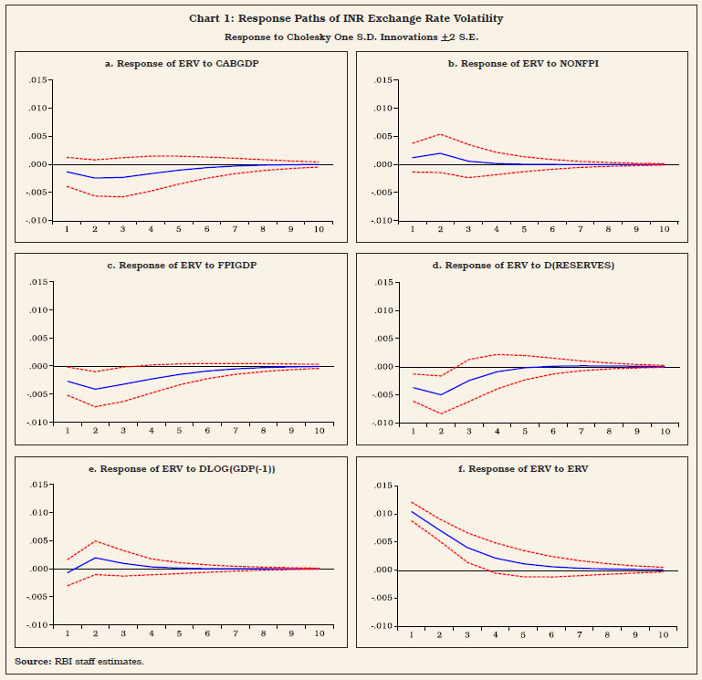
“… WHEREAS it is essential to have a modern monetary policy framework to meet the challenge of an increasingly complex economy.” [Excerpted from Preamble to the Reserve Bank of India (RBI) Act, 1934 1. Introduction V.1 As India’s experience in the lead-up to the institution of flexible inflation targeting (FIT) vividly showed, persistently high inflation can carry the seeds of external vulnerabilities, which surged to a crescendo during the taper tantrum in the summer of 2013. High inflation morphed into a balance of payments crisis, posing a severe challenge to monetary policy credibility (Patra, 2017). For an open emerging market economy, surges, sudden stops and reversals in capital flows and related volatile exchange rate movements complicate the conduct of monetary policy in the short run. By influencing domestic liquidity and monetary conditions, they feed into domestic inflation, depending on the degree of exchange rate pass-through (ERPT) to domestic prices and the effectiveness of sterilisation operations. Over the longer run, persistently high levels of inflation tend to erode export competitiveness and along with imported inflation can worsen the terms of trade and the current account balance. V.2 In an open economy setting, therefore, policy authorities are confronted with ‘impossible’ trade-offs, requiring them to sacrifice one of three policy choices: monetary policy independence; exchange rate stability; and an open capital account (Mundell, 1963; Fleming, 1962). The rapid globalisation of economies and the cross-border integration of domestic financial markets have amplified these challenges. In fact, irrespective of the exchange rate regime, financial openness has posed complications for independent conduct of monetary policy, morphing the trilemma into a dilemma, a choice between capital mobility and independent monetary policy (Rey, 2013). In the aftermath of the global financial crisis (GFC), global spillovers of unconventional monetary policies (UMPs) of systemically important central banks added a new dimension to the open economy policy trade-offs, i.e., domestic financial conditions became heavily influenced by interest rate settings in advanced economies (AEs) and the slosh of global liquidity which impacted credit spreads, risk premia, credit flows and leverage, rendering the pursuit of domestic monetary policy objectives even more challenging. Countries with fixed/managed exchange rate regimes found that they are more likely to experience financial vulnerabilities – faster domestic credit and housing price growth, and increases in bank leverage – than those with relatively flexible regimes (Obstfeld et al., 2017). In this complex international environment, emerging market economies (EMEs) have brought to bear several innovations in the conduct of open economy monetary policy. They have resisted depreciation with a combination of foreign exchange interventions and interest rate defences; they have learnt over time to manage appreciation pressures better, using a combination of sterilised interventions, capital flow management measures (CFMs) and macro-prudential policies. As a result, EMEs have transformed the dilemma in practice to an asymmetric 2.5 lemma (Cheng and Rajan, 2019). The most important innovation brought in by EMEs has been the happy marriage between FIT and foreign exchange intervention. This can be characterised as an intermediate approach between the two ‘impossible’ corner solutions – fixed exchange rate versus fully open capital account – in the conduct of monetary policy. As a result, the practice of monetary policy in EMEs has moved ahead of theory (BIS, 2019). The global narrative today is all about developing a consensus on an integrated policy framework (IMF, 2019; Adrian and Gopinath, 2020). V.3 Since the adoption of FIT in India in June 2016, India has also used its own intermediate approach to deal with global spillovers, absent any multilateral consensus on an ideal framework. This chapter covers India-specific issues relating to managing open economy challenges and trade-offs under FIT. Section 2 provides stylised facts on India’s openness, comparing the FIT experience with that of the pre-FIT period. Section 3 drills down into underlying exchange rate dynamics, including the effectiveness of sterilised interventions in enhancing flexibility in the conduct of monetary policy in India, and nuances of exchange rate pass-through to domestic inflation. Section 4 summarises policy responses with the help of an open economy Taylor type rule to guide the setting of monetary policy amidst UMPs and global spillovers, taking into account implications for current account sustainability and competitiveness. Section 5 summarises the findings and ends with key takeaways and policy inferences. 2. Openness: Some Stylised Facts V.4 Despite various de jure policies that have sustained the progressive liberalisation of the capital account in India, cross-border capital flows as a ratio to GDP have moderated during the FIT period (Chart V.1). This reflects a global pattern among EMEs (Chart V.2). At the global level, growing trade protectionism and the retrenchment of banking sector flows largely explain the moderate levels of trade related and capital flows in the post-GFC period. In the case of India, deceleration in the rate of domestic capital formation has also constrained productive absorption of foreign capital. 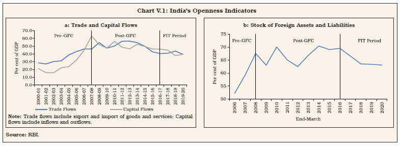 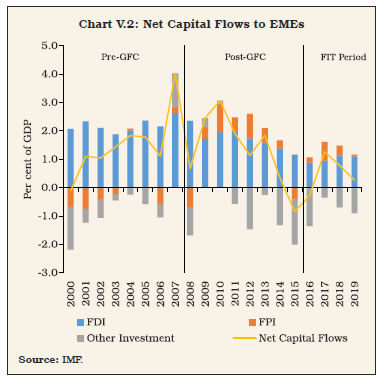 V.5 On the other hand, India’s external vulnerability indicators have improved dramatically, allowing for greater independence of monetary policy from global developments (Table V.1). In particular, the current account balance, the bellwether indicator of India’s external viability in view of the historical predominance of trade and remittances in the country’s external interface, has strengthened, benefitting from low oil prices during the FIT period and net terms of trade (ToT) turning favourable in 2019-20 (Chart V.3). 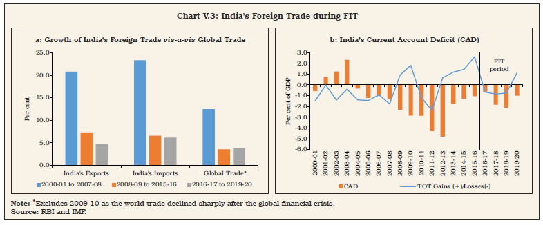 V.6 Net capital inflows exceeded CAD funding requirements during the FIT period. The Indian economy, thus, experienced the problem of poor absorption of saving from abroad that could have complemented domestic savings and worked as a lever for stepping up the pace of growth in a time of abundant global liquidity and ultra-low interest rates. The result was overall balance of payments surpluses and an unprecedented accumulation of India’s official reserves (Table V.2). This assumes relevance in comparison with the pre-GFC period when capital inflows averaged about 4.1 per cent of GDP per annum during 2000-01 to 2007-08, coinciding with a phase of high domestic investment rates that peaked at 37.7 per cent of GDP in 2007-08. V.7 Volatility in capital flows – both gross and net – declined during the FIT period in terms of both standard deviations over a rolling window of four quarters (Engle et al., 2008; Broto et al., 2011; Eichengreen et al., 2017; and Pagliari and Hannan 2017) and standard deviations of residuals obtained from an auto-regressive moving average (ARMA (1, 2)) model to check for the presence of any ARCH effects1 (Val and Libanio, 2009; Pagliari and Hannan, 2017) (Chart V.4).2 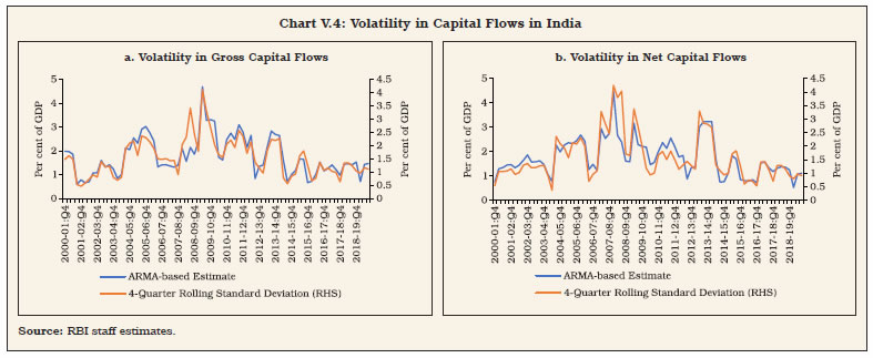 3. Exchange Rate Dynamics and FIT V.8 EMEs have been late movers in the adoption of FIT in view of large exogenous effects of exchange rate volatility on inflation and price competitiveness, embodied in the ‘fear of floating’ (Calvo and Reinhart, 2002) and ‘fear of appreciation’ (Levy-Yeyati and Sturzenegger, 2007). This also reflected their large dependence on trade in goods and services and the existence of less developed financial markets (Cavoli, 2009). In practice, most of the EMEs and some AEs have resorted to frequent and large interventions in the foreign exchange market to deal with the challenges arising from excessive capital flows and the associated impact on exchange rate volatility (BIS, 2005; IMF, 2011; Berganza and Broto, 2012). 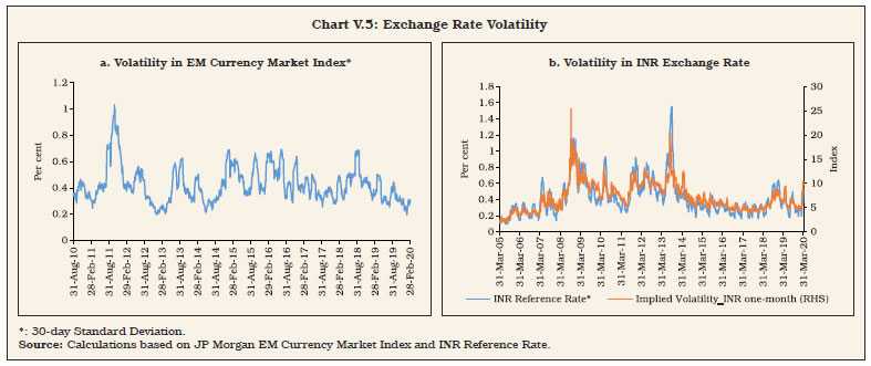 V.9 In India, exchange rate policy aims at containing excessive volatility, without any pre-specified target or band for the Indian rupee (INR). With the decline in volatility of capital inflows (as highlighted in the previous section and Chart V.4), the INR has also exhibited stability during the FIT period (Chart V.5). In India, changes in capital flows emerge as one of the key forces influencing INR volatility (Box V.1).
V.10 The sensitivity of INR to monetary policy changes – in India and abroad (in the US as a representative numeraire) – can be examined through the covered and uncovered interest rate parity conditions. The empirical literature on this subject, however, remains divided, with some views emphasizing the role of higher interest rates in attracting foreign capital which, in turn, leads to appreciation of the domestic currency (Dornbusch 1976, Frankel 1979 and Christiano et al. 1998), and others interpreting interest rate differential as an indicator of rising inflation, which must reflect in depreciation of the domestic currency in due course (Mussa 1979 and Bilson 1978, 1979). In India, the co-movement between interest rate differentials (based on three-month treasury bill rates in India and the US) and the INR (Chart V.6) does not provide empirical support for uncovered interest rate parity (UIP).3 The covered interest rate parity is more directly verifiable and holds for the INR in the behaviour of forward premia (Chart V.7). Empirical estimates of determinants of the INR find weak evidence of any role for interest rate differentials; instead global VIX, an indicator of global risk aversion, emerges as a statistically significant determinant (Box V.2). 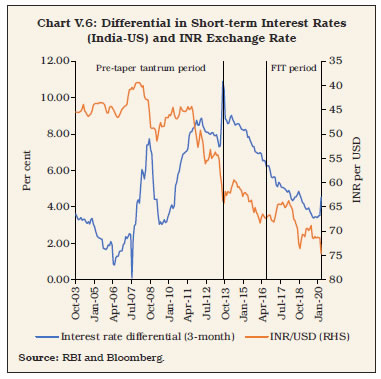 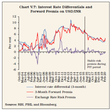 V.11 Given the dominant role of capital flows in exchange rate volatility in India and the offset provided by reserve accumulation, it is inevitable that monetary policy design gets strongly influenced by the choice between non-sterilised interventions (and associated implications for domestic liquidity conditions) versus sterilised interventions (with associated implications for yields and forward premia). While unsterilised interventions can create surplus liquidity that can depress short-term interest rates to levels lower than the policy interest rate, sterilisation of surplus liquidity through open market operations (OMOs) can influence longer-term yields while the use of swaps to delay the liquidity impact of intervention could alter forward premia. Intervention operations to manage volatility in the exchange rate can thus pose challenges for monetary policy independence by influencing the term structure of interest rates.
V.12 Intervention operations alter the size and composition of the Reserve Bank’s balance sheet. Sterilisation is conditioned by the size of domestic securities’ holdings available with the Reserve Bank for conducting OMOs to absorb surplus liquidity. During the FIT period, the share of net foreign assets (NFA) has declined below 75 per cent of the Reserve Bank’s balance sheet from around 85 per cent before the global financial crisis, creating space for sterilisation to manage the liquidity impact of interventions (Chart V.8). Besides, the high share of NFA induced the Reserve Bank to use multiple instruments such as market stabilisation scheme and cash reserve ratio in addition to open market sales operations for sterilisation purposes. 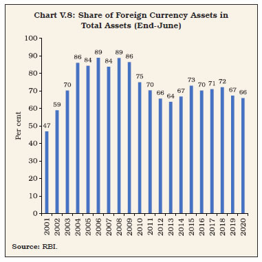 V.13 In some years, such as in 2017-18, net open market sales were undertaken to sterilise surplus liquidity (Table V.3). In 2018-19, however, a decline in NFA led to contraction in domestic liquidity and hence, the Reserve Bank conducted large open market purchase operations to counter the impact of lower NFA on liquidity and also to meet the normal incremental demand for primary liquidity in the economy. In 2019-20, open market purchases were undertaken to supplement the rupee liquidity generated from forex operations in order to first ensure easy financial conditions to counter the slowdown and in the context of the pandemic towards the close of the year. V.14 Open market sales for sterilisation can harden yields which, in turn, can attract more yield-differential sensitive capital inflows and cause further addition to liquidity, eventually making sterilisation ineffective. Accordingly, updated estimates of the sterilisation coefficient and the offset coefficient become useful for policy purposes (Box V.3). The sterilisation coefficient indicates the extent of change in net domestic assets (NDA) in the balance sheet of the Reserve Bank that results in response to the change in the NFA. The offset coefficient indicates the change in NFA in response to the NDA-induced change in yields. Both the coefficients vary between 0 and -1. A sterilisation coefficient reaching close to -1 indicates a situation of full sterilisation of the liquidity generated from forex interventions, leaving the reserve money level unchanged. The sterilisation coefficient, however, does not convey anything on the effectiveness of sterilisation. This is given by the offset coefficient – a value close to -1 indicates perfect capital mobility, making sterilisation operations completely ineffective. On the other hand, an offset coefficient closer to zero helps in preserving monetary policy independence through sterilised interventions. In India, the size of the estimated offset coefficient has increased during the FIT period to -0.3 from about -0.2 in the pre-FIT period, but remains well below -1, thereby establishing sterilised intervention as an effective instrument for preserving monetary policy independence.
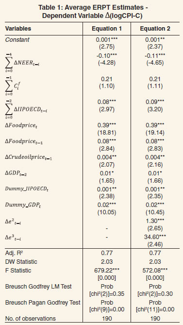
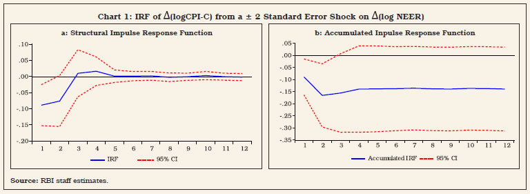
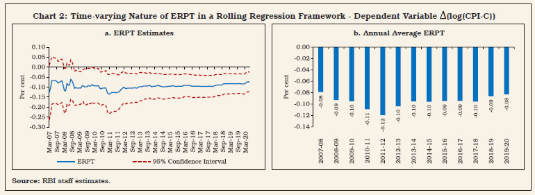
Pass-Through of Exchange Rate Changes to Inflation V.15 The sensitivity of inflation to exchange rate shocks has a more direct implication for the effectiveness of monetary policy. Since the exchange rate is neither an instrument of policy nor an intermediate target under FIT, a precise assessment of exchange rate pass-through to domestic inflation provides a forward-looking dimension to guide the implementation of monetary policy. In several IT practicing countries, experiences characterised by high volatility in the exchange rate and large pass-through effects may require explicit incorporation of exchange rate shocks as an additional determinant of flexibility within the FIT framework, whether in terms of the tolerance band or the time horizon over which the inflation target could be achieved. V.16 Available estimates of ERPT for India mostly relate to WPI/CPI-IW inflation (Table V.4). Two estimates which relate to CPI-C inflation suggest an ERPT coefficient of 0.15 over five months (Patra et al., 2018) and 0.10 over four months (Kundu, 2019). Updated estimates of ERPT for India using alternative approaches suggest a range of 0.10 to 0.13, with a gradual decline in ERPT during the FIT period (Box V.4). V.17 Taking into account the stylised facts in Section 2 and the characteristics of underlying inflation dynamics in an open economy in Section 3, this section turns to the implementation of rule-based inflation targeting in an open economy drawing on seminal work (Svensson, 1997; Ball, 1997). In an open economy, monetary policy transmits through both the interest rate and the exchange rate. Accordingly, any monetary policy rule should take into account: (i) the role of real exchange rate changes in explaining output (through net exports) and inflation (through pass-through of import prices to domestic prices and inflation expectations) and (ii) the role of the interest rate in influencing movements in the exchange rate. V.18 An open economy monetary policy rule, which has attracted intuitive practitioner appeal, can be defined in the form of a monetary conditions index (MCI) (Ball, 1999):  The MCI is measured as a weighted sum of changes (per cent) in the short-term real interest rate relative to a base period and changes in the real effective exchange rate index relative to a base period. The MCI has been used by some inflation targeting central banks such as the Bank of Canada and the Reserve Bank of New Zealand as a short-term operational reference variable. The Bank of Canada generates short-term quarterly paths for desired MCI values, consistent with the quarterly inflation path. In some other countries like Sweden, Norway, Finland and Iceland, the MCI was used as one of several indicators for forming the policy stance (Gerlach and Smets 2000). The estimated MCI for India indicates that monetary conditions remained tighter during the FIT period than in the pre-FIT period (Chart V.9).6 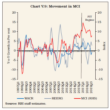
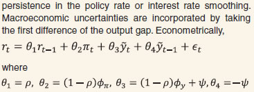
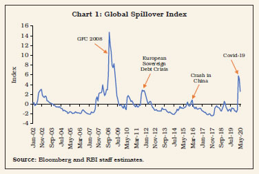
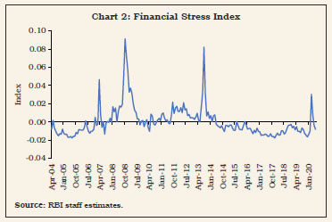
V.19 The MCI is a statistical construct and is unobservable. Moreover, it is confined to monetary conditions as narrowly defined by the joint movements in the interest rate and the exchange rate. In order to set monetary policy, however, a broader array of macroeconomic and financial conditions need to be evaluated to determine the path of the policy instruments. For India, an open economy Taylor rule has been estimated with a global spillover index (GSI) that is constructed on the basis of the sensitivity of domestic financial markets to global financial stress/spillovers (Box V.5), nominal/real effective exchange rates, the federal funds rate and a composite indicator of domestic financial stress that combines pressures in four markets – equity, bond, forex and money – by using a dynamic factor model. Empirical estimates show that while both the inflation gap and output gap play statistically significant roles in determining the path of the policy interest rate, neither the exchange rate nor the federal funds rate seems to have any statistically significant influence on monetary policy rate decisions in India. Monetary policy is, however, found to be sensitive to both global spillovers and domestic financial stress.
V.20 India’s observed pattern in capital flows to GDP ratio during the FIT period reflects the generalised moderation in capital flows to EMEs. Compared with interest rate differentials, time varying risk premium – which is a function of global as well as domestic factors – appears to be a major driver of INR volatility. The monetary policy rate is not found to respond directly to exchange rate movements or the federal funds rate, although the conduct of monetary policy is sensitive to financial shocks, both global and domestic. Estimates of ERPT suggest some moderation during the FIT period, but inflation can still alter by 10-13 per cent of the change in exchange rate, warranting that the exchange rate be closely monitored as a key information variable for the conduct of monetary policy. V.21 Sterilised intervention is an effective solution to manage the trilemma in India. Enhancement of sterilisation capacity may be necessary to deal with possible surges in capital flows in future. Activation of the standing deposit facility (SDF) can address the security availability constraint of RBI for undertaking sterilisation operations, but market-based sterilisation instruments are required to avoid misalignment of the operating target relative to the policy repo rate. Adequate provisions for market stabilisation scheme (MSS) securities in the Union Budget every year may be necessary to strengthen monetary operations of the RBI, consistent with the level of international reserves that is considered conducive for managing exchange rate volatility. The precautionary requirements for building adequate buffers against global spillovers is a public policy objective, and not confined to the realm of monetary policy alone. V.22 In the absence of budgetary allocations of marketable securities for the conduct of monetary policy in an open economy context, lessons can be drawn from the practice of several central banks that issue their own securities to effectively pursue goals set for monetary policy in the face of large autonomous increase in surplus liquidity due to capital flows. Globally, many advanced country central banks, such as Switzerland, Japan and Sweden issued their own securities to absorb surplus liquidity in the aftermath of GFC. Among the EMEs which have adopted an inflation targeting framework, the Bank of Indonesia pioneered the use of central bank securities even before the Asian financial crisis of 1997. Other inflation targeting central banks which issue their own securities include Thailand, Mexico, Israel, Peru and Chile. For a majority of central banks, their respective legislations allow them to issue their own securities. The option of issuance of its own securities by the RBI, currently prohibited under section 19(5) of the RBI Act 1934, may be explored by amending the Act suitably. V.23 Sustained accretion to foreign exchange reserves in recent years has improved reserve adequacy in terms of conventional metrics such as cover for imports and short-term debt. Reserve cover for imports is still lower, however, than other major reserve holding economies. Moreover, in an extremely stressed environment in which external obligations become callable, about half of the reserves can be potentially encumbered for repayment of short-term debt by residual maturity (i.e., falling due over the next twelve months) (Annex V.1). Going by the post-taper tantrum experience, i.e., sudden shifts in market assessment of adequacy and self-fulfilling multiple equilibria in the exchange market, the foreign exchange reserve buffer needs to be strengthened further. V.24 Looking ahead, the emergence of INR as an international currency appears inevitable. While greater internationalisation of the INR can lower transaction costs of cross-border trade and investment operations by mitigating exchange rate risk, it can also complicate the conduct of monetary policy. Internationalisation of a currency makes the simultaneous pursuit of exchange rate stability and a domestically oriented monetary policy more challenging, unless supported by large and deep domestic financial markets that could effectively absorb external shocks. By broadening the scope for both residents and non-residents to buy and sell domestic currency denominated financial instruments, internationalisation can potentially limit the ability of the central bank to control domestic money supply and influence interest rates as per domestic macroeconomic conditions. V.25 Besides deep and sophisticated financial markets, the most important pre-requisite for internationalisation of a currency is price stability. Inflation, higher than the world average, undermines the use of a currency as an international medium of exchange and a store of value and can restrict the role of such an economy in global value chains. While high inflation disincentivises cross-border trade and investment by enhancing the cost of acquiring information for pricing, stable prices build confidence of international investors in the domestic currency. In India, the primary focus of FIT on price stability augurs well for further liberalisation of the capital account and internationalisation of the INR. References: Aizenman, J., Chinn, M., and Ito, H. (2010a), “The Financial Crisis, Rethinking of the Global Financial Architecture, and the Trilemma,” Asian Development Bank Institute Working Paper No. 213 (April). Aizenman, J., Chinn, M., and Ito, H. (2010b). “The Emerging Global Financial Architecture: Tracing and Evaluating the New Patterns of the Trilemma’s Configurations”, Journal of International Money and Finance, Vol. 29, No. 4, pp. 615–641. Aizenman, J., Chinn, M.D., Ito, H. (2013), “The “Impossible Trinity” Hypothesis in an Era of Global Imbalances: Measurement and Testing,” Review of International Economics, Wiley Blackwell, Vol. 21(3), pp.447-458, August. Aizenman, J., Chinn, M.D., Ito, H. (2008), “Assessing the Emerging Global Financial Architecture: Measuring the Trilemma’s Configurations over Time”, NBER Working Paper Series No. 14533. Aron, J.; R. Macdonald and J. Muellbauer (2014), “Exchange Rate Pass-Through in Developing and Emerging Markets: A Survey of Conceptual, Methodological and Policy Issues, and Selected Empirical Findings,” The Journal of Development Studies, Vol. 50, No. 1, pp.101-143. Tobias Adrian and Gita Gopinath (2020), “Toward an Integrated Policy Framework for Open Economies”, https://blogs.imf.org/2020/07/13/toward-an-integrated-policy-framework-for-open-economies/. Ball, Laurence (1997), “Efficient Rules for Monetary Policy”, National Bureau of Economic Research Working Paper No. 5952. Ball, Laurence (1999), “Policy Rules for Open Economies”, available at http://www.nber.org/chapters/c7415.pdf Bank for International Settlements (2005), “Foreign Exchange Market Interventions in Emerging Markets: Motives, Techniques and Implications.” BIS Papers No. 24. Bank for International Settlements (2014), “Emerging economies respond to market pressure”, BIS Quarterly Review, March. Bank for International Settlements (2019), Monetary policy frameworks in EMEs: inflation targeting, the exchange rate and financial stability” Annual Economic Report 2019. Berganza, Juan Carlos and Carmen Broto (2012), “Flexible inflation targets, forex interventions and exchange rate volatility in emerging countries”, Journal of International Money and Finance, Vol. 31 (2012), pp. 428–444. Bhattacharya, R.; I. Patnaik and A. Shah (2008), “Exchange Rate Pass-through in India,” Macro/ Finance Group at NIPFP, Available at: <https://macrofinance.nipfp.org.in/PDF/BPS2008_erpt.pdf> Bilson, John F. O. (1978), “The Monetary Approach to the Exchange Rate: Some Empirical Evidence”, IMF Staff Papers, Vol. 25(1), pp 48-75. Bilson, John F. O. (1979), “The deutsche mark/ dollar rate : A monetary analysis,” Carnegie-Rochester Conference Series on Public Policy, Vol. 11(1), pp. 59-101. Broto, C.; Díaz-Cassou, J. and Erce, A. (2011), “Measuring and explaining the volatility of capital flows to emerging countries”, Journal of Banking & Finance, Vol. 35(8), pp.1941-1953. Calvo, G., Reinhart, C. (2002), “Fear of floating”, Quarterly Journal of Economics, Vol. 117, pp.379–408. Cavoli, T. (2009), “Is fear of floating justified? The East Asia experience”, Journal of Policy Modeling, Vol. 31, pp.1–16. Cheng, Ruijie and Ramkishen S. Rajan (2019), “Monetary trilemma, dilemma, or something in between?”, International Finance, Vol.23, pp.257–276. Choudhri, E. U. and D. Hakura., (2006), “Exchange Rate Pass-through to Domestic Prices: Does the Inflationary Environment Matter?” Journal of International Money and Finance, Vol. 25, No. 4. Christiano, L. J., M. Eichenbaum, and C. L. Evans (1998), “Monetary Policy Shocks: What Have We Learned and to What End?” Working Paper No. 6400, National Bureau of Economic Research. Dornbusch, R. (1976), “Expectations and exchange rate dynamics”, Journal of Political Economy, Vol. 84, pp.1161–1176 Dua, Pami and Partha Sen (2006), “Capital Flow Volatility and Exchange Rates: The Case of India”, CDE Working Paper No.144. Eichengreen, B; P Gupta, and O Masetti (2017), “Are Capital Flows Fickle? Increasingly? And Does the Answer Still Depend on Type?”, World Bank Policy Research Paper No. 7972. Engel, Charles (2016), “Exchange Rates, Interest Rates, and the Risk Premium”, American Economic Review, 106 (2), pp.436-74 Engle, R. F. and Rangel, J. G. (2008), “The Spline-GARCH Model for Low-Frequency Volatility and Its Global Macroeconomic Causes”, Review of Financial Studies, Vol. 21(3), pp.1187-1222. Fleming, J.M. (1962), “Domestic Financial Policies Under Fixed and Under Floating Exchange Rates,” Staff Papers, International Monetary Fund, Vol. 9 (November), pp.369–79. Frankel, J.A. (1979), “On the mark: a theory of floating exchange rates based on real interest differentials”, American Economic Review, Vol. 69, pp.610–622. Gerlach, Stefan, and Franks Smets (2000), “MCIs and monetary policy in small open economies under floating exchange rates” European Economic Review, Vol. 44, pp. 1677-1700. Ghosh, A. and R. S. Rajan., (2007), “How High is Exchange Rate Pass-through in India? Has it Changed over Time?” The Journal of International Trade and Economic Development, Vol. 16, No. 3, pp.373-382. International Monetary Fund (2011), World Economic Outlook, April, IMF Washington, D.C. International Monetary Fund (2019), Statement by the Managing Director on the Work Program of the Executive Board Executive Board Meeting, June 3. Jiménez‐Rodríguez, R., and A. Morales‐Zumaquero (2020), “BRICS: How important is the exchange rate pass‐through?”, The World Economy, Vol. 43, No. 3, pp.781-793. Kapur, M. (2012), “Inflation Forecasting: Issues and Challenges in India,” RBI Working Paper Series, No. 01. Kapur, M. and H. Behera (2012), “Monetary Transmission Mechanism in India: A Quarterly Model,” RBI Working Paper Series, No. 9. Khundrakpam, J. K. (2007), “Economic Reforms and Exchange Rate Pass-through to Domestic Prices in India,” BIS Working Papers, No. 225. Kohli, R (2015), “Capital Flows and Exchange Rate Volatility in India: How Crucial Are Reserves?”, Review of Development Economics, Vol.19, No.3, pp.577–591. Koustas, Z., and Lamarche, J.-F. (2012), “Instrumental variable estimation of a nonlinear Taylor rule”, Empirical Economics, Vol. 42(1), pp.1–20. Kundu, S. (2019), “The Impact of Exchange Rate Changes on Consumer Prices: Evidence from India”. In D. Finck and P. Tillmann (Eds.), Price-setting Behaviour and Inflation Dynamics in SEACEN Member Economies and their Implications for Inflation (The SEACEN Centre, pp. 87-125). Levy-Yeyati, E., Sturzenegger, F. (2007), “Fear of appreciation”, KSG Working Paper 07-047, Harvard University. Mundell, R.A. (1963), “Capital Mobility and Stabilization Policy under Fixed and Flexible Exchange Rates”, The Canadian Journal of Economics and Political Science, Vol. 29, No. 4 (Nov., 1963), pp. 475-485. Mussa, Michael (1979), “Empirical regularities in the behavior of exchange rates and theories of the foreign exchange market”, Carnegie-Rochester Conference Series on Public Policy, Vol. 11, pp.9-57. Obstfeld, M., Ostry, J., Qureshi, M. (2017), “A Tie That Binds; Revisiting the Trilemma in Emerging Market Economies”, IMF Working Paper 17/130. Pagliari, Maria Sole and Swarnali Ahmed Hannan (2017), “The Volatility of Capital Flows in Emerging Markets: Measures and Determinants”, IMF Working Paper No.17/41. Patra, M. D. and M. Kapur, (2010), “A Monetary Policy Model without Money for India,” IMF Working Paper No.10/183. Patra, M. D.; J. K. Khundrakpam and A. T. George, (2014), “Post-Global Crisis Inflation Dynamics in India: What has Changed,” India Policy Forum (2013-14), NCAER, pp.117-191. Patra, M. D.; S. Pattanaik; J.J and H. K.Behera (2016), “Global Spillovers and Monetary Policy Transmission in India”, RBI Working Paper Series, No. 03/2016. Patra, M. D., (2017), “One Year in the Life of India’s Monetary Policy Committee,” Reserve Bank of India – Speech, October 27. Patra, M.D.; J.K. Khundrakpam and J.John (2018), “Non-Linear, Asymmetric and Time Varying Exchange Rate Pass-Through:Recent Evidence from India”, RBI Working Papers Series, No.2. Rafi, O. P. C. Muhammed and M. Ramachandran (2018), “Capital Flows and Exchange Rate Volatility: Experience of Emerging Economies”, Indian Economic Review, Vol.53, pp.183-205. Rey, H (2013), “Dilemma not trilemma: the global financial cycle and monetary policy independence”, proceedings of the Federal Reserve Bank of Kansas City Jackson Hole symposium, August 2013. Sen Gupta, A. and R. Sengupta (2013), “Management of Capital Flows in India”, ADB South Asia Working Paper Series, No. 17, Asian Development Bank. Smets, F., and Wouters, R. (2007), “Shocks and frictions in US business cycles: A Bayesian DSGE approach”, American Economic Review, Vol. 97(3), pp.586–606. Stock, J.H. and Mark W. Watson (2016), Handbook of Macroeconomics, Volume 2A, Elsevier. Svensson, L. E. O (1997), “Inflation forecast targeting: implementing and monitoring inflation targets”, European Economic Review, Vol. 41, pp.1111-46. Taylor, John B (1993), “Discretion versus Policy Rules in Practice,” Carnegie Rochester Conference Series on Public Policy, Vol. 39, pp.195-214. Val, Vanessa da Costa and Gilberto Libanio (2009), “Capital Flight or Volatile Financial Flows: which one is the best indicator to measure Brazilian External Vulnerability?”, paper presented at AHE Annual Conference 2009. 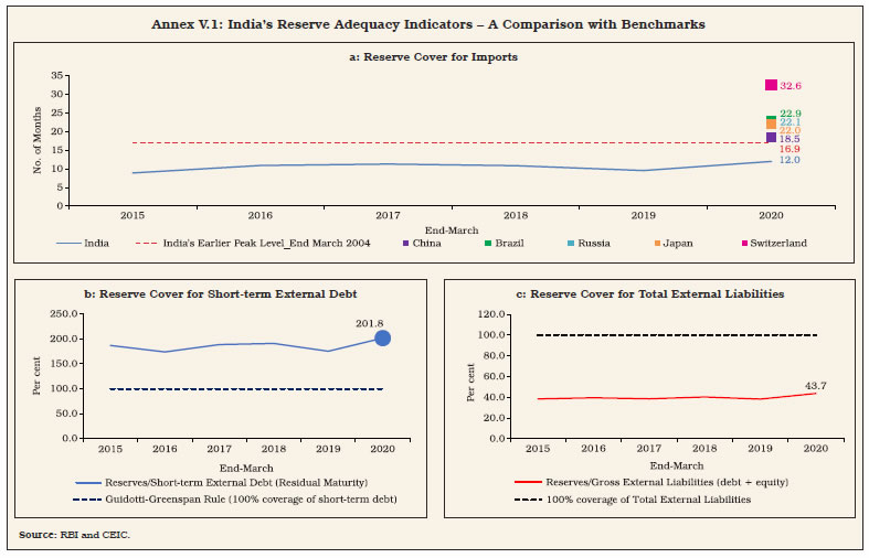 This Chapter has been prepared by a team comprising Rajeev Jain, Amarendra Acharya, Soumasree Tewari, Manu Sharma, Sujata Kundu, Silu Muduli, Shobhit Goel and Rohan Bansal. 1 ARCH effects refer to the phenomenon of volatility or variance clustering, where periods of high volatility are followed by periods of higher volatility and period of low volatility are followed by periods of lower volatility. 2 Quarterly data for the period 2000-01:Q1 to 2019-20:Q3 (as per cent of GDP) are used. 3 UIP theory states that the difference between interest rates between two economies should equal the expected change in exchange rate (rather than observed change in exchange rate) to nullify any opportunity for arbitrage gains. 4 The study uses pd as measured by the CPI-C published by the CSO under the MoSPI, GoI. e is represented by NEER (based on trade-based weights) published by the RBI. The indicator of foreign price/cost conditions is constructed as: cƒ = NEER*CPI-C/REER. yd is proxied by the CSO’s quarterly real GDP series. Using the Denton method on the seasonally adjusted index of industrial production (IIP) of the CSO (taking average IIP as the indicator), the quarterly real GDP series at market prices was converted to a monthly series. IIP of the OECD countries available from the OECD statistics is used to incorporate yƒ. pc is proxied by the global average crude oil prices available from the World Bank Commodity Price Data (The Pink Sheet). Average crude oil prices are also treated as a proxy for domestic cost conditions. CPI-IW food is used for food prices. Variables were converted into their natural logarithms and were seasonally adjusted by the US Census Bureau X-13 ARIMA programme. The lag selection was done through the Schwarz Criterion (SC), Akaike Information Criterion (AIC), and the Hannan-Quinn Criterion (HQC). All variables were stationary at first differences. Dummy variables for IIPOECD and GDP were used to take into account the impact of the global financial crisis (2008-09 to 2010-11). 5 According to Ball (1999), π* stands for (π+γe-1) where π is inflation, e is log of real exchange rate, y is log of real output and r is real interest rate. 6 The weights w and 1-w for weighted average call rate and real effective exchange rate in MCI are estimated to be 0.65 and 0.35, respectively, and the overall MCI ratio works out to 1.83. A 1 percentage point change in the real interest rate has about the same effects over time on real aggregate demand as a 1.83 percentage point change in the real effective exchange rate. 7 In order to identify global spillovers, a composite global spillover index (GSI) is constructed following Patra et al. (2016) with the following five global spillover variables in standardised form (i) VIX, an indicator of risk aversion of the foreign investors; (ii) LIBOR-OIS spread, an indicator of liquidity stress in the overseas market and risk of default in short-term lending; (iii) DXY- the dollar index, capturing the exchange rate channel of global spillovers; (iv)Term-spread, or the difference between 10-year US treasury bill yield and 3-month US treasury bill yield; and (v) Risk-spread, which is the 10-year US treasury bill yield subtracted from 10-year US corporate bond yield. A dynamic factor model (DFM) is used to estimate the GSI for India (Stock and Watson, 2016). The constructed GSI for India captures reasonably well the various phases of stress in global financial markets and their spillover to Indian markets (Chart 1). A high value of GSI indicates turbulence in the global financial markets. The financial stress index (FSI), which is also used in the Taylor rule, reflects a composite measure of stress in various domestic financial market segments at any point in time (Chart 2). The FSI is constructed capturing both source of stress, i.e., external versus domestic. |
صفحے پر آخری اپ ڈیٹ:


