Media, as an important channel for dissemination of information, has the potential to influence public sentiment and expectations. This article utilises high frequency unstructured information sourced from the online print media, in the specific context of retail inflation in India. Using Support Vector Machines (SVM) classifier, a widely used technique for sentiment classification, sentiment is extracted from the news and a sentiment index is constructed. Empirical results suggest that the media sentiment index tracks inflation very well. Its directional accuracy, is high and statistically significant. Further, the Granger Causality test results also indicate that the sentiment index has significant predictive ability for retail inflation.

Introduction

Media, as an important channel for dissemination of information, has the potential to influence public sentiment and expectations, which could have important interlinkages with macro-economic outcomes. Using Big Data techniques, the information content in such new data, is being exploited by researchers worldwide to construct appropriate alternative indicators which could help predict macro-economic variables. This article contributes to this growing literature by analysing media sentiment in the specific context of retail inflation in India.

In order to analyse high-frequency and large volume of unstructured information, it is imperative to deploy Big Data tools, such as Machine Learning (ML) and Natural Language Processing (NLP) techniques. Using SVM classifier, a widely used technique for sentiment classification, sentiment is extracted from the news. We utilise unstructured news text sourced from online print media news and reports, in the specific context of retail inflation in India. Availability of such high frequency information (daily news) offers the advantage to construct an index on a near-real time basis.

Against this backdrop, an attempt is made to (i) extract sentiment contained in news on inflation, (ii) aggregate sentiments and construct a sentiment index, and (iii) examine empirically the relationship between sentiment and inflation.

The remainder of this article is structured as follows. Section II briefly reviews the relevant literature. The methodology of sentiment classification and construction of a sentiment index is described in Section III. Empirical results examining the relationship between media sentiment and inflation is presented in Section IV, and Section V concludes.

II. Review of Literature

Newspaper information based indices have been constructed and used in various macroeconomic and financial analysis such as economic policy uncertainty (Baker et al., 2016; Bhagat et al., 2013), financial market movements (Baker et al., 2019; Manela and Moreira, 2017), expected evolution of macro-economic variables (Beckers et al., 2017; Shapiro et al., 2017) and central bank related likely policy response (Lamla and Sturm, 2013; Hendry, 2012; Tobback et al., 2017). We briefly review a few studies specific to the analysis of inflation.

Consumers’ reaction to the information provided by media is throughly examined in literature. Common people may not have full understanding of the macroeconomic models, and also they may not track the latest statistics, and instead they may rely on news media for the latest updates on macroeconomic developments to build their forecasts and form their expectations. Thus, media as a transmitter of news may have direct impact on inflation expectations of households (Carroll, 2003). Reaction of consumers to the information provided by news media may be influenced by both quantity (coverage of news) and quality (tone of news) (Lamla and Lein, 2008).

Media news is found to be associated with heterogeneity in inflation expectations of consumers, the reporting intensity and news content may play an important role (Lamla and Maag, 2012). Media is found to be a significant influencer in addition to various socio-economic characteristics which act as possible determinants of inflation expectations (Ehrmann et al., 2017). Taking a slightly different route, some studies focus on linkage of news sentiment and business cycle indicators. It is found that use of news sentiment improves the forecasting performance of the model (Beckers et al., 2017; Shapiro et al., 2017).

III. Methodology for Sentiment Classification and the Sentiment Index

Online data sources provide an opportunity to exploit news, which are voluminous and are in unstructured text format, making it challenging for manual reading and processing. In the literature, three broad approaches are used for sentiment analysis using raw news text, viz. dictionary based approach, semantic orientation and machine learning techniques.

Dictionary based methods (such as Loughran-McDonald dictionary) for sentiment classification are easy to understand and implement, which have been applied in economics and finance (Iglesias et al., 2017, Nyman et al., 2018). While such methods are useful to extract general sentiment contained in the text, they may not be appropriate for context specific sentiment as they are generic in nature and not well defined for a particular context (such as inflation).

Semantic Orientation (SO) approach tries to address the issue of specific context, as a researcher can provide a list of pre-defined keywords exogenously, as considered appropriate for a given context. Following the user provided keywords, the SO approach aims to measure the degree of positivity or negativity in a given text (Lucca and Trebbi, 2009; Turney, 2002; Tobback et al., 2017). The SO approach is straightforward and easy to adopt; however, it has certain limitations, such as high dependency on keywords and possible bias (Tobback et al., 2017).

The issue of providing appropriate keywords exogenously by the researcher is resolved by using Machine Learning (ML) methods. These methods automatically search for words/ patterns in given text documents which would distinguish one sentiment class from another, and are being used in recent periods (Tobback et al., 2017; Shapiro et al., 2017). SVM, a supervised machine learning technique, is a widely used method in sentiment classification.

III.1 Sentiment Classification - Methodology

We collect news from online print media, focussing on retail inflation in India. Information extraction and sentiment classification methodologies are fairly developed for english language and, therefore, we limit our scope to english news in this article. One may think of exploring and extracting sentiment from news in other Indian languages as well, to check possible variations in sentiment on account of language (if any). However, english being a widely used language in print media across states/ regions in India, we believe that the sentiments extracted from news written in english would be reasonably representative.

As SVM classifier is a supervised model¹, labelled documents with distinct features and input in the form of a document-term matrix (DTM) are pre-requisites for training the model². In the present case, each news item was considered as a unique document and the words mentioned in the news served as terms.

Sentiment was assigned to each news item (increase, decrease or neutral) by thoroughly reading the news text. Some of the news could not be classified into one of the three sentiment classes (i.e. there was no sentiment related to inflation), and were, therefore, labelled as “nil”. This process resulted in all documents getting labelled in one of the four classes/ categories, viz. “increase”, “decrease”, “neutral” or “nil”.

We describe the entire process from data collection to sentiment classification, by way of a flow chart (Chart 1), details are in Annex I.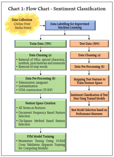

The underlying concept used in SVM is to identify specific features which can be used to distinguish one sentiment class from another, and, therefore, only a few documents having the right mix of features can serve the purpose, by reducing the noise and improving the accuracy of the classification model.

Hence, feature selection methods are often used in sentiment analysis to select specific features which are comparatively more informative and would aid in achieving higher classification accuracy. The basic idea is to rank the features according to certain measures and remove non-informative features. We have explored two measures, viz. document frequency based and the Chi-square approach for feature selection. Details are provided in Annex II. Thus, in addition to the basic model with all features, two more variants of the model were trained following the two feature selection methods.

As is the usual practice for machine learning algorithms, to verify the model performance, data were segregated into train and test data and an optimal model from various competing models is selected based on the performance metric namely “accuracy ratio” in test data. Accuracy ratio is a standard evaluation metric/ measure for classification models, which represents the ratio of correctly classified observations to the total observations. A model with higher accuracy ratio (in test data) is considered better among the competing models.

The corpus was segregated into train and test data set in 70:30 ratio, and Table 1 indicates the proportion of the news items in train and test data.

As could be observed from Table 1, only a few observations are present in “neutral” class, leading to an unbalanced data problem. This is a common scenario in qualitative survey results (categorical data) and also in cases where the target variable is continuously changing (in either direction) and the possibility of the variable remaining in the same state is rather very low.

One approach to handle unbalanced data is to combine the low observation class with another (adjacent) class, one may think of merging “neutral” class with either “increase” or “decrease”. In this article, however, this approach was not considered, as construction of a sentiment index (at later stage) requires three classes (“increase”, “decrease” and “neutral”).

Separate models are trained and tested with different feature space, as described earlier (Table 2). In the second model, even if the number of features are comparatively much lower than the first model, the accuracy improved a lot, highlighting the fact that working with suitable features gives better results. Therefore, the second model was chosen as the optimal model for sentiment classification as its accuracy was higher compared to other models in test data. Using Model 2, sentiment was assigned to all news items, from April 2015 to March 2019.

III.2 Sentiment Index - Methodology

After classifying documents (news items) under four sentiment classes, viz. “increase”, “decrease”, “neutral” and “nil”, the next step is to aggregate them and derive an overall sentiment for each period of time. Inflation changes from one period of time to another (little or more) and the possibility of it being same over two consecutive time periods is rather very low. Hence, the possibility of news items with “neutral” sentiment is expected to be rather very low. Yet, to cover all the aspects of sentiment, we count all such news items in the corpus. News items categorised as “nil” are discarded in the computation of the sentiment index as they do not convey any sentiment and their inclusion could result in an inaccurate index.

Measuring news sentiment is somewhat analogous to qualitative business tendency surveys, which aim at measuring sentiment/ expectations of target survey respondents. The survey responses are generally aggregated using Net Response, which is the difference between “increase” and “decrease” responses (proportions). We construct a Sentiment Index (SI) as defined below:

where I_t = number of news items with ”increase” sentiment in time period t

D_t = number of news items with “decrease” sentiment in time period t

N_t = total number of news items (increase, decrease and neutral)

The SI ranges between (-)100 to (+)100, where a negative value of the index indicates decrease in inflation and a positive value indicates increase in inflation.

Availability of daily news facilitates calculation of the SI on a daily basis, thereby making it a high frequency indicator. However, for the purpose of assessment vis-à-vis official monthly inflation numbers, we compute the SI for each month, taking into account all days in a month.

At the same time, we do not want to lose any significant information contained in daily news. So, we try to combine certain days of the month and re-compute the SI. Inflation being one of the keenly watched macro-economic variable, is frequently reported in media. However, its coverage increases more around the time of the release of official data on Consumer Price Index (CPI) inflation.

Against this backdrop, we combine days of each month into three distinct sets, as defined below:

Set 1 : Day 1 to T-1

Set 2 : Day T to T+2

Set 3 : Rest of the month,

where T = date of issue of the press-release on monthly CPI data, which may vary slightly at times, from month to month

Hence, we calculate four SI values for each month, one for each date Set (Set 1, Set 2 and Set 3) and an overall monthly index including all days of the month. The goal is to explore possible differences in sentiment on inflation, if any, owing to the timing of the arrival of the news. This categorisation of news into sets is advantageous in the following aspects:

(i) Less computation, time-specific sentiment;

(ii) Early availability of sentiment, well before the completion of month; and

(iii) If the sentiment of a particular Set is better linked to inflation, we may not need to consider other days, which may be of advantage.

III.3 Stylised Facts on the Sentiment Index

In this section, the typical characteristics of the sentiment index are described, at aggregate and disaggregated level. Distribution of news items according to the sentiment in each month is presented in Chart 2. One may observe that the proportion of news classified as “neutral” is almost negligible for most of the months (this is in line with expectation, given the fact that the target variable, i.e. inflation, is continuously changing). Further, in each month, the majority of news is primarily focused on either “increase” or “decrease” sentiment class, and the instances when both types of sentiments are equally prevalent in media is rare. Such concentration of media sentiment implies clarity in sentiment formation, and results in a high negative or high positive value of the Sentiment Index.

The distribution of news items, with respect to the three date sets is presented in Chart 3.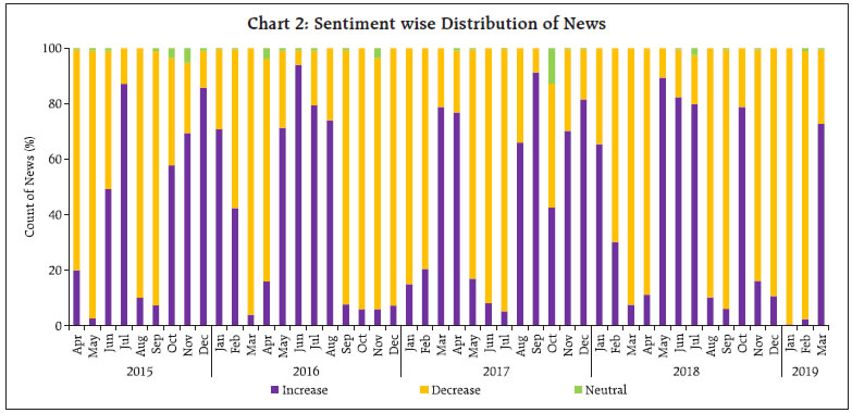

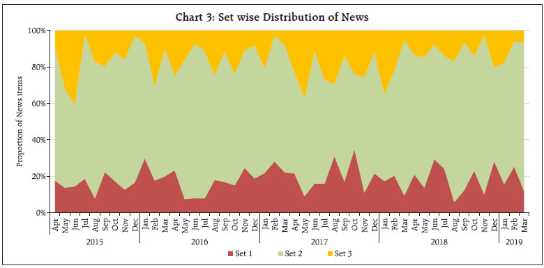
It could be observed that even though Set 2 consists of only 3 days of the month, most of the news items are captured during this period, as compared to other days in a month. It is quite understandable as a lot of deliberations on the current inflation trends and the likely future path of the indicator takes place around the date of the official release of inflation data.

It would be interesting to see whether the coverage of more news during Set 2 has any role to play in the overall sentiment for the month. We plot the overall Sentiment Index against each Set (Chart 4 to Chart 6). While the index based on Set 2 is better reflective of the index of all dates, the same is not observed for index of Set 1 and Set 3. The coverage of more news in Set 2, combined with possibly better sentiment coverage, might have contributed to a high degree of co-movement between the index of Set 2 and the index of all dates.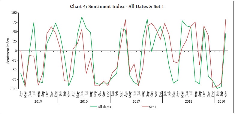

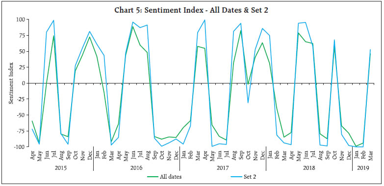
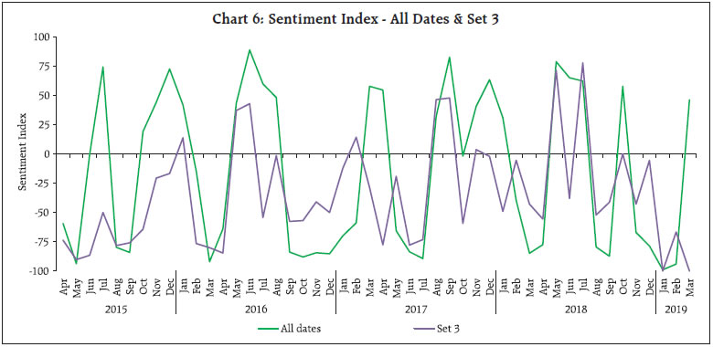
IV. Empirical Analysis

The constructed sentiment index is available almost a fortnight before the release of official CPI data. Additionally, the sentiment Index pertaining to Set 2 is available almost a month before the release of data on inflation. As english news has been considered for deriving the sentiment, which may be read in mostly urban parts of the country, the sentiment index may possibly be better related to urban inflation. On the other hand, since newspapers usually report about similar issues at any given point in time, in various languages, the index may as well be linked to rural inflation. So, we consider the combined, urban and rural inflation in this article.

We define inflation as the annual change in logarithmic values of CPI. Since the sentiment index indicates the direction of change in inflation, we define monthly change in inflation as below:

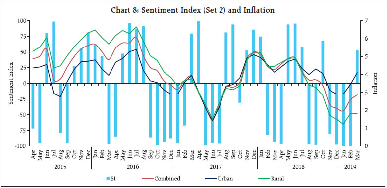
where CPI_i,t = CPI of class i in period t,
(i = C for Combined, i = U for Urban, i = R for Rural)

Data from April 2015 to March 2019 has been considered in the current analysis. We begin with graphical, correlation and directional analysis before testing for causality.

IV.1 Graphical and Correlation Analysis

A high degree of co-movement is observed between the sentiment index and inflation, indicating that the sentiment index is able to track directional changes in inflation reasonably well (Chart 7 and Chart 8).

Correlation analysis reveals that sentiment is strongly and significantly correlated with inflation. The correlation is somewhat weaker for rural inflation as compared to urban inflation, but statistically significant. Linkage of SI of Set 2 with inflation is stronger, while Set 1 and Set 3 sentiment indices do not appear to be significantly correlated with inflation (Table 3).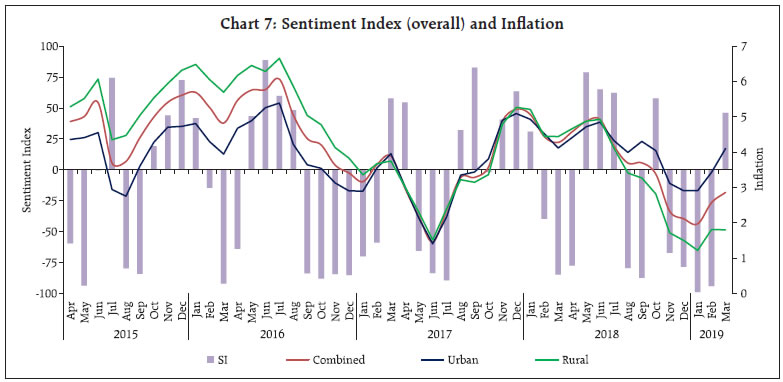

IV.2 Directional Analysis

Directional analysis is adopted to evaluate the tracking performance of sentiment index in capturing the turning points in inflation. There are several standard directional metrics, we use “accuracy”, the simplest and widely used metric in related literature. It is generally defined as the proportion of instances when the predicted class matches with the reference class. In our case, it is defined as the proportion of time periods (months) when the direction indicated by the sentiment index matched with the direction of change in inflation.

A positive SI indicates increase in inflation while a negative SI indicates decrease in inflation. For each month, sign of SI and sign of Δπ (change in inflation) is noted, and number of months is counted for each pair of directional change to create a 2 x 2 contingency table, using which accuracy is computed (Table 4).

A high accuracy score implies that SI is able to capture the directional change in inflation very well.

We also use Fisher’s Exact (FE) test to examine the directional accuracy. Using the contingency table (Table 4), the null hypothesis whether the direction given by the sentiment index and direction of change in inflation are independent, is tested. A rejection of the null hypothesis implies that the SI is useful in capturing the direction of change in inflation.

where, N = A+B+C+D

The observed significance level of FE test is defined as below,

As observed earlier, in addition to the overall SI, Set 2 SI appears to be closely associated with inflation, and therefore, we consider overall SI and Set 2 SI for directional analysis.

The results of directional measures, viz. Accuracy and FE test are presented in Table 5.

With accuracy of 65 per cent, the sentiment index appears to capture the directional change in inflation reasonably well, both for combined and urban inflation. The accuracy is comparatively lower for rural inflation. The FE test reconfirms the significant association between sentiment and inflation, except rural inflation.

IV.3 Causality Analysis

Presence of causality is important to examine predictive ability. The Granger Causality test is often used in the literature to check the presence of causal relationship between two variables. The underlying hypothesis is that lagged values of a variable explain the variation in another variable and vice-versa.

As observed earlier, in addition to the overall SI, Set 2 SI appears to be closely associated with inflation, and therefore, we consider overall SI and Set 2 SI for causality test.

We estimate following pairs of equations for Granger Causality test:

Where SI and Δπ are sentiment index and change in inflation as defined in equations (1) and (3) above. Subscript i indicates type of inflation (combined, urban or rural), whereas subscript j denotes type of SI (o and 2 for Overall and Set 2, respectively).

The null hypothesis - of βκ are jointly zero - is tested and its rejection confirms that SI Granger-Causes Δπ. Similarly, rejection of the null hypothesis - of γκ are jointly zero - confirms that Δπ Granger-Causes SI. The lag selection (value of n) is done using Schwarz Information Criteria (SIC).

We test for the presence of unit root in both variables, SI and Δπ, before performing the Granger Causality test, in order to ensure that variables are stationary. Augmented Dickey Fuller test (ADF) and Phillips-Perron test (PP) are used, where rejection of null hypothesis would confirm stationarity of the variables. The unit root tests suggest that the sentiment index and change in inflation are stationary (Table 6).

The Granger Causality test indicates presence of bi-directional causality between sentiment and change in inflation (Table 7).

It is evident from the results of Granger Causality test that inflation, besides its own lags, is also influenced by sentiment, and vice-versa. Thus the sentiment index has significant explanatory power for predicting inflation.

V. Conclusion

This article uses high frequency unstructured information reported in the media and employs Big Data techniques to construct a sentiment index, with the objective of (a) constructing alternative indicators that could be useful to assess the state of the economy, on a near real-time basis, and (b) improving nowcasting of inflation based on use of media information.

Harnessing the power of Machine Learning and Natural Language Processing techniques, specifically SVM classifier, sentiment has been extracted from unstructured text (news) to construct a sentiment index. Empirical results suggest that the media sentiment index tracks inflation very well. Its directional accuracy, is high and statistically significant. Further, the Granger Causality test results also indicate that the sentiment index has significant predictive ability for inflation.

References

Baker, S. R., Bloom, N. and Davis, S. J. (2016), “Measuring economic policy uncertainty”, The Quarterly Journal of Economics, 131(4), 1593-1636.

Baker, S. R., Bloom, N., Davis, S. J. and Kost, K. J. (2019), “Policy News and Stock Market Volatility”, National Bureau of Economic Research (NBER) Working Paper No. 25720

Beckers, B., Kholodilin, K. A. and Ulbricht, D. (2017), “Reading between the Lines: Using Media to Improve German Inflation Forecasts”, German Institute for Economic Research, Discussion Papers 1665

Bhagat, S., Ghosh, P. and Rangan, S P. (2013), “Economic Policy Uncertainty and Economic Growth in India”, Indian Institutes of Management (IIM) Bangalore Working Paper No. 407

Carroll, C. D. (2003), “Macroeconomic Expectations of Households and Professional Forecasters”, The Quarterly Journal of Economics, 118(1)

Chakraborty, C., and Joseph, A. (2017), “Machine learning at central banks”, Bank of England, Working Paper No. 674

Ehrmann, M., Pfajfar, D. and Santoro, E. (2017), “Consumers’ Attitudes and Their Inflation Expectations”, International Journal of Central Banking

Hendry, S. (2012): “Central Bank Communication or the Media’s Interpretation: What Moves Markets?” Bank of Canada, Working Paper 9

Iglesias, J., Ortiz, A. and Rodrigo, T. (2017), “How do the Emerging Markets Central Bank talk? A Big Data approach to the Central Bank of Turkey”, BBVA Economic Research Department Working Paper, 17-24

Lamla, M. J. and Lein, S. M. (2008), “The Role of Media for Consumers’ Inflation Expectation Formation”, Swiss Economic Institute (KOF) Working Paper, No. 201

Lamla, M. J. and Maag, T. (2012), “The Role of Media for Inflation Forecast Disagreement of Households and Professional Forecasters”, Journal of Money, Credit and Banking, Vol. 44, No. 7

Lamla, M. J. and Sturm, J. E. (2013), “Interest rate expectations in the media and central bank communication,” KOF Working Paper, No. 334

Lekshmi, O. and Mall, O.P. (2015), “Forward looking surveys for tracking Indian economy: an evaluation”, Bank for International Settlements (BIS) Irving Fisher Committee (IFC) Bulletin No. 39

Loughran, T. and McDonald, B. (2011), “When is a Liability not a Liability? Textual Analysis, Dictionaries, and 10-Ks”, Journal of Finance, 66, 35-65.

Lucca, D. O. and Trebbi, F. (2009), “Measuring Central Bank Communication: An Automated Approach with Application to FOMC Statements”, NBER Working Paper No. 15367

Manela, A. and Moreira, A. (2017), “News implied volatility and disaster concerns” Journal of Financial Economics, 123, 137-162

Nyman, R., Kapadia, S., Tuckett, D., Gregory, D., Ormerod, P. and Smith, R. (2018), “News and narratives in financial systems: exploiting big data for systemic risk assessment”, Bank of England Working Paper No. 704

Picault, M. and Renault, T. (2017), “Words are not all created equal: A new measure of ECB communication”, Journal of International Money and Finance 79, 136–156.

Shapiro, A. H., Moritz, S., and Wilson, D. (2017), “Measuring News Sentiment”, Federal Reserve Bank of San Francisco, Working Paper 01

Tobback, E. and Nardelli, S. and Martens, D. (2017), “Between Hawks and Doves: Measuring Central Bank Communication”, European Central Bank (ECB) Working Paper No. 2085

Turney, P. D. (2002), “Thumbs Up or Thumbs Down? Semantic Orientation Applied to Unsupervised Classification of Reviews”, Proceedings of the 40th Annual Meeting on Association for Computational Linguistics (pp. 417-424).

Annex I - Sentiment Classification

The raw news collected from online print media is suitably cleaned by removing Uniform Resource Locator (URL), special characters and symbols, punctuation and numerals. Common stop words¹ along with some custom stop words, which do not provide any specific value for sentiment classification, were also removed.

Words are often used with different variations in the text for the purpose of readability depending on the grammar with underlying meaning being the same. In order to create single feature from many similar meaning words, the words are normalised to their root forms. We used lemmatisation², a process which converts each word into its lemma, which is an actual language word. Proper care is taken of grammar, vocabulary and dictionary importance of a word while doing the conversion.

The lemmatised news is then tokenised into unigrams (individual term), resulting in a set of terms for each document, for the entire corpus.

Terms are weighted using Term Frequency - Inverse Document Frequency (TF-IDF) weight, as defined below:

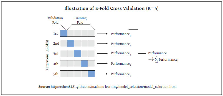
where TF_ij = number of times term i occurs in document j

DF_i = number of documents containing term i

N = total number of documents

The TF-IDF weight is a measure used frequently in textual data to evaluate the importance of a term in a given corpus. A term is assigned high weight if it occurs frequently in a document (by TF) but is offset by the number of documents in the corpus that contain the word (by IDF) resulting in balanced weight.

Although SVM can handle non-linear decision boundaries, given the nature of data, we use linear SVM in this article. The linear SVM classification model is a maximum margin classifier and has the following form:

f(x_j)=w₀ + w_1j x_1j+ w_2j x_2j+... + w_njx_nj

where w_ij = weight of term i in document j

x_ij = occurence of term i in document j

w₀ = intercept

The sign of the resulting decision function f(x_j) is the predicted class of a particular document.

The weights of the decision function are a function only of a subset of the training data set, called support vectors. Those are the data points that are closest to the decision boundary and lie on the margin. The weights of various terms are obtained while training the model. Since we have a four-class classification problem, six one-v/s-one binary sub-classifiers are built, and the final sentiment class is selected based on maximum votes.

The misclassification cost on training data is based on cost parameter C. Large value of C makes the cost of misclassification high, whereas a small value of C can result in low misclassification error. An optimal value of C is required, which can be achieved using parameter tuning. In the present case, an optimal value of C has been obtained using K-fold cross-validation with K = 10, details are as follows:

K-Fold Cross-Validation

• Randomly split the train dataset into K “folds”

• For each K-fold (validation), build model on K-1 folds of the dataset

• Then, test the model to check the effectiveness for K^th fold

• Record the performance (error) of each of the predictions

• Repeat this until each of the K-folds has served as the validation set

• The average of K recorded errors is called the cross-validation error and serves as performance metric for the model

_________________________________________________________

¹ Stop words are natural language words, which occur frequently in text, however convey little meaning to the text, for example, “the”, “a”, “and”, “this”, “are” etc. We used english stop words from SMART (“System for the Mechanical Analysis and Retrieval of Text”) which contains a widely used set of stopwords in textual analysis.

² R package TEXTSTEM was used for lemmatization.

Annex II - Feature Selection Method

(i) Document Frequency based measure - In text documents, it is a common phenomenon to get terms which are not often used in all the documents. The terms (features) may be ranked based on the respective document frequency (i.e. proportion of documents in which the particular term appears). Using a threshold value, some terms which are ranked lower may be excluded. We have used the threshold value as 0.005, implying that all the terms which appear in less than 0.5 per cent of the documents are excluded.

(ii) Chi-Square measure - Chi square statistic χ² measures the association between a feature and a class. Using a contingency table containing the count of news as cell frequency as indicated below, χ2 is computed and p-value is obtained. A significant χ2 value implies that the related class is more associated with the given feature. Features which are not found to be significantly associated with related class (at 1 per cent level of significance) have been discarded.

* This article is prepared by Shweta Kumari and Geetha Giddi, Department of Statistics and Information Management (DSIM), Reserve Bank of India (RBI). The views expressed in this article are those of the authors and do not represent the views of the Bank. The errors, if any, are those of the authors.

¹ A very brief explanation of SVM is provided in this article, for details one may refer to Chakraborty and Joseph, 2017.

² We use CARET package in R for SVM model training and testing.