Press Release

RBI Working Paper Series No. 20
Credit Channel of Monetary Transmission in India - How Effective and Long is the Lag?
^@Jeevan Kumar Khundrakpam

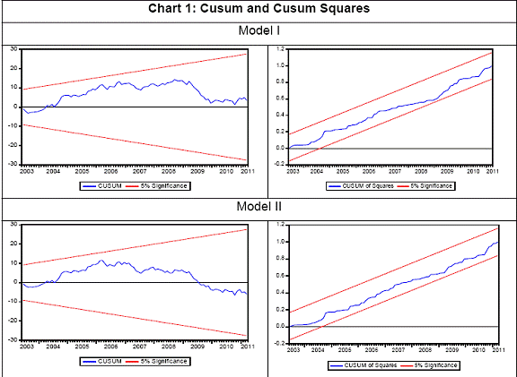
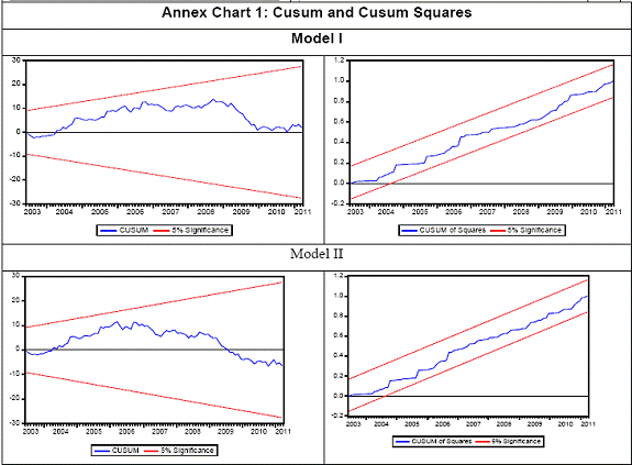
Abstract

^*This paper examined the operation of credit channel of monetary policy rate transmission in India during the post-LAF period of 2001:3 to 2011:3. Drawing on the literature, two reduced form equations, one representing nominal bank credit and the other real bank credit was estimated. The regression estimates were carried out after transforming the variables to stationary form and following an approach similar to Hendry’s general-to-specific method. Stability and structural break tests were performed, and rolling regressions were estimated to confirmed robustness of the results.

It finds that, besides the positive influence of economic activity on bank credit, policy induced expansion or contraction in deposit or money supply makes banks to adjust their credit portfolio correspondingly. Importantly, the credit channel of monetary transmission is found to be significant and robust. Specifically, the transmission of policy rate to nominal or real bank credit growth takes about seven months over the full sample period as well as across various sub-sample periods. Over the full sample period, 100 basis points increase in policy rate was found to reduce the annualised growth in nominal and real bank credit by 2.78 per cent and 2.17 per cent, respectively.  However, a decline in the magnitude of the impact of policy interest rate on bank credit has been observed during the post global financial crisis period.

Keywords: Monetary Transmission, Bank Credit, Policy Rate

JEL Classification Codes: E51, E52

Introduction

Monetary policy framework in India has undergone a significant shift, particularly with the adoption of liquidity adjustment facility (LAF) as the operating procedure of monetary policy. Consequently, since the beginning of the 2000s, change in policy interest rate has occupied the central role in signaling the stance of monetary policy. Needless to say, the effectiveness of this interest rate signals in the achievement of ultimate monetary policy objectives of growth with price and financial stability would depend on how the signals are transmitted through the financial system and the economy, and how businesses and households react. In general, there are mainly four transmission channels of monetary policy, viz., commercial interest rates, asset prices, the exchange rate and expectations. Among these, the commercial interest rate is often the main channel of transmission. In this channel, change in policy interest rate affects the deposits and lending rates of financial institutions, and alters the spending and investment decisions of households and businesses, and consequently inflation and growth.

In view of the increasing role assigned to interest rate as the monetary policy instrument, this piece attempts to explore whether the credit channel of transmission of policy rate in India is effective and what has been the lag in transmission. Drawing on the theoretical literature, two reduced form equations are derived based on which the regression equations are estimated after examining the time series properties of the variables and converting them to stationary form. Specifically, controlling for other determinants, we estimate the lag impact of policy rate on nominal and real bank credit following an approach similar to Hendry’s general-to-specific method. The consistency and robustness of the estimated equation in terms of lag structure of the variables across sub-sample periods are then confirmed by conducting structural break tests and employing rolling regression technique.

The rest of the paper is organised as in the following. Section I is a review of the literature briefly listing out the approaches and some of the empirical findings. The model specification is spelled out in Section II. Section III explains the series to be used and analyses their properties. The empirical results are analysed in section IV. The final section provides the concluding remarks.

Section I. Review of Literature

In the literature, the effectiveness of monetary policy on bank lending is founded on the premise that i) there are borrowers who are dependent on banks and ii) monetary policy directly affects willingness of banks to lend. The existence of borrowers dependent on banks is derived from the theory of credit market imperfections. For instance, small firms are less informed of credit conditions and have lesser array of financing options than large firms. Thus, the dependence of small firms on bank credit is more than that of large firms (Diamond, 1984; Marsh, 1982). Consequently, empirical analysis on demand for bank credit is often carried out by differentiating the credit behavior of small and large firms. Empirically, small firms are found to be much more severely affected by monetary tightening than large firms as they have less access to bank and non-bank external finance (Gertler and Gilchrist, 1994; Oliner and Rudebusch, 1994).

Monetary policy affecting willingness of banks to lend is examined either by analysing the portfolio adjustment behavior of banks or the impact on price and non-price term of lending of banks. With regard to portfolio adjustment behavior, the hypothesis is that monetary policy changes alter the bank transactions deposits or core deposits, which after some lags lead to decline in bank loans (Bernanke and Blinder, 1992: Romer and Romer, 1990). However, the empirical evidence on monetary policy tightening affecting bank portfolio behavior, and then lending, has not been unambiguous. For instance, Gertler and Gilchrist (1993) examining from the point of view of demand for loan by small and large firms find that monetary tightening has no effect on business lending. In contrast, examining the lending or supply of credit of small and large banks, Kashyap and Stein (1995) find that monetary policy tightening affects the lending of small banks, but not the lending by large banks. These conflicting results could follow as banks balance sheets approach contain no information about impact of rate changes on new loans, besides the  possibility that change in balance sheet is due to factors such as non-performing loans rather than  having to do anything with monetary policy.

Thus, monetary policy impact on bank lending is also analysed by examining the role of price and non-price term in bank lending. Under this approach there are two explanations on the bank credit channel of monetary transmission viz., lending view and credit rationing. According to lending view, when there is policy tightening, the volume of new loan should decline and loan rates should rise relative to market rates. In contrast, credit rationing theory suggest that the decline in volume on new loan following monetary policy tightening should be accompanied by bank loan rates increasing less than the market rate.

In the Indian context, there are some empirical studies showing the existence of bank lending channel of monetary policy. Panditet. al (2006) using a VAR framework on quarterly panel data of banks for the period 1997 to 2002 find that the changes in cash reserve ratio (CRR) and the Bank Rate get transmitted to bank lending channel, with the impact being far more severe on small banks than large banks.  Similarly, Virmani (undated) using a VAR framework for the period April 1992 to March 2002 also finds the evidence of change in monetary base getting transmitted to credit channel. These studies, however, pertain to pre-LAF period with change in monetary base as the main policy instruments.

For the post-LAF period of the 2000s, Bhaumik et. al (2010) using annual panel data of banks for 2000 to 2007 examined the implications of bank ownership on transmission of monetary policy to supply of bank credit. They find that there are considerable differences in the reactions to monetary policy initiatives of various banks differentiated by ownership pattern. These reactions are also influenced by the surplus or deficit liquidity conditions, with bank lending channel of monetary policy transmission being more effective under deficit condition than under surplus condition. However, instead of repo or reverse repo rate, the study considered the prime lending rates announced by the individual banks as the monetary policy interest rate.

More recently, Pandit and Vashisht (2011) examined the transmission of policy rate viz., repo rate from the perspective of demand for bank credit in India. Using monthly data during January 2001 to August 2010 in a panel framework of seven emerging market economies including India they find change in policy interest rate to be an important determinant of firm’s demand for bank credit. Thus, they conclude that monetary policy is an important countercyclical tool for setting the pace of economic activity in India.

In our present context, the credit channel of transmission of monetary policy is examined under equilibrium condition of demand and supply of credit at an aggregated level of all banks. Unlike Pandit and Vashisht (2011) who considered repo rate as the policy rate, we consider the weighted call rate as the proxy for policy rate. This is because in India the effective policy rate had alternated between repo and reverse repo rate depending upon the deficit or surplus liquidity conditions. Therefore, it would be incorrect to consider repo rate alone as the policy rate. Weighted call rate, on the other hand, had mostly hugged the effective policy rate between the repo and reverse repo rate as the liquidity situation changed. Further, our focus is more on identifying the lag at which the change in policy interest rate gets transmitted to bank credit channel and robustness of that lag.

Section II. Model Specification

The model is an eclectic adaptation of the Ehrmannet. al (2001), which draws on the model of Bernanke and Blinder (1988), and Kashyap and Stein (1995). The supply of bank credit (C_j^s) is defined as a function of the available amount of deposits (D) or money (M), nominal interest rate on credit (r) and directly the monetary policy rate (i). This direct impact of policy rate on supply of bank credit arises as it is assumed that either bank uses the interbank market to finance their loans or follows mark-up pricing that deposit rates are passed on to lending rates. Thus, loan supply is given by,

C_j^s = α₁D + α₂r + α₃i                                                              (1)

In Ehrmann et. al (2001), it is assumed that the dependence of banks on deposits for supply of loan depends on the size or liquidity of a bank. In particular, the lower the size or liquidity of a bank the smaller is the impact of change in deposits on supply of credit. In our case, for simplicity, we assume that the dependence of bank credit on deposit is homogenous across banks and, therefore, size neutral. This assumption has been made for the sake of simplification so that the impact of monetary policy on bank credit could be analysed at the aggregated level of all banks.

The demand for bank credit (C_j^d) which a bank faces depends on real economic activity (Y), price level (P), nominal interest rate on credit (r) and nominal exchange rate (e) as,

C_j^d = α₄Y + α₅P + α₆r + α₇e                                                  (2)

Real economic activity is assumed to have a positive impact on demand for loan, while nominal interest rate has a negative impact. It is assumed that the interest rate elasticity of demand for credit is independent of bank size. Inflation can either have a positive or a negative impact on credit demand. When firms make use of both money and bank loans for working capital finance, high inflation penalises money holding and makes bank loans more attractive. On the other hand, high inflation by reducing productivity and reducing demand for labour lowers the demand for bank credit by firms (Cukierman and Hercowitz, 1989). The impact of nominal exchange rate on credit demand can also be either negative or positive. An exchange rate appreciation by increasing the relative return on external financial assets over investment in real domestic assets can reduce financing gap and demand for bank credit. On the other hand, credit demand could increase due to exchange appreciation to finance acquisition of the more attractive external financial assets (Vera, 2003).

The nominal interest rate on credit is then assumed to be affected by change in policy interest rate with some lags. Thus,

r = α₈i                                                                                      (3)

Combining (1) to (3) under the equilibrium condition of demand and supply for bank credit, we arrive at the following reduced form equation,

C_t = β₀ + β₁Y_t + β₂D_t + β₃P_t + β₄e_t + β₅i_t + ε_t                                               (4)

Where we define the variables as in the following

C_t           = Nominal bank credit in period t
Y_t           = Level of real economic activity in period t
D_t           = Nominal bank deposits or money supply in period t
P_t           = Price in period t
e_t           = Nominal exchange rate in period t
i_t            =  Central bank nominal policy rate at time t
ε_t           = Error term in period t

Equation (5) is essentially a reduced form equation of supply for aggregate bank credit, but augmented with variables determining demand for bank credit. These demand determining variables have been included in order to control for demand shocks so that cyclical movements in credit is captured and the impact of monetary policy component of interest changes on supply of bank credit is isolated (Kashyap and Stein, 1995). 

In equation (5), all the variables are in nominal term, except the real income variable. This follows from the segregation of nominal income variable into its price and real components to distinguish between the price and income elasticity of bank credit. This is the most common practice in the literature where, following Bernanke and Blinder (1988) and Kashyap and Stein (1995), the estimation of bank credit channel of monetary policy transmission is carried out using nominal variables¹.

Few studies, however, estimate demand/supply of bank credit in real terms using real explanatory variables. But, they still continue to use policy interest rate in nominal terms (e.g., Farinha & Margues, 2002; Pandit & Vashisht, 2011). One important reason for using nominal interest rate while other variables are in real terms follows from the difficultly in constructing an expected inflation series. Consequently, real interest rate which is defined as nominal interest rate minus expected inflation rate is not easily derivable.  Thus, following the practice in the literature, in addition to (4), we also derive a reduce form equation in real terms, except for the policy rate which continues to be in nominal terms as²,

RC_t = γ₀ + γ₁Y_t + γ₂RD_t + γ₃re_t + γ₅i_t + ε_t                                                     (5)

Where we define the variables as in the following

RC_t       = Real bank credit in period t
Yt         = Level of real economic activity in period t
RD_t       =Real bank deposits or money supply in period t
re_t         = Real exchange rate in period t
i_t           =Central bank nominal policy rate at time t
ε_t          =Error term in period t

In the following, in order to establish the robustness of credit channel of monetary policy rate transmission in India, we, therefore, estimate two models: i) Model I, represented by reduced form equation (4); and ii) Model II, represented by equation (5).

Section III. Data and Properties

The data used in this study are of monthly frequencies for the period 2001:3 to 2011:3 culled out from Real Time Handbook of Statistics on Indian Economy, Reserve Bank of India. Essentially, we capture the period since the introduction of Liquidity Adjustment Facility (LAF) as the operating procedure of monetary policy, when interest rate became the main monetary policy signaling instrument. Even though data are available beyond March 2011, we do not consider them as recent trend suggest that they are likely to undergo substantial changes, particularly the index of industrial production (IIP) and wholesale price index (WPI).

Nominal bank credit (C) is the total non-food credit of scheduled commercial banks. As GDP data are not available at monthly frequencies, we have considered IIP as proxy for real economic activity. Price is measured by WPI. Exchange rate is measured by 36-country trade weighted nominal effective exchange rate (NEER). Nominal deposit (DEP) includes all types of deposits of scheduled commercial banks, while nominal money supply is measured by broad money measure (M₃). Weighted average call rate (CallR) is used as proxy for policy rate, as it has tended to hug the effective policy rate – repo rate or reverse repo rate – depending upon the liquidity condition. To arrive at the real bank credit (RC), real deposit (RDEP) and real money supply (RM3), the corresponding nominal series were deflated by WPI. For real exchange rate, 36-country trade weighted real effective exchange rate (REER) has been considered.

All the variables are converted to natural logarithm. They have not been seasonally adjusted in order to capture the information containing in their seasonal behavior. In India, credit demand has a clear seasonal pattern and monetary policy is adapted to the need of this seasonality in credit demand. Therefore, de-seasonalising of the variables will lead to significant loss of information.

Unit Roots Tests

The ADF and PP tests results presented in table-1 reveal the following. Credit, deposit and money supply, both in nominal and real terms, viz., C, RC, DEP, RDEP, M3 and RM3,  are all unambiguously non-stationary. On the other hand, call rate (CallR) and both nominal and real effective exchange rate (NEER and REER) are stationary. With regard to index of industrial production (IIP) and price (WPI), the two tests show contradictory results, but unambiguously stationary in first difference form.

Unit root tests thus reveal that residual based cointegration analysis cannot be carried out, as they are not integrated of the same order. On the other hand, OLS regression in level form will be spurious as most of the variables are non-stationary. Thus, we estimate the regressions for the two models in first difference or growth form, except call rate, which are all stationary, and therefore, will not be spurious. In other words, the regression equations for the two models, respectively, take the following forms.

∆logC_t = β₀ + β₁∆logIIP_t + β₂∆logDEP_t + β₃∆logWPI_t + β₄∆logNEER_t + β₅logCallR_t +ε_t       (6)
∆logRC_t = γ₀ + γ₁∆logIIP_t + γ₂∆logRDEP_t + γ₃∆logREER_t + γ₄logCallR_t+ε_t                        (7)

Section IV. Empirical Results

Regression Results

In estimating the regression, we followed an approach similar to Hendry’s general-to-specific method. First, the maximum lag length of the variables was set at 11, as they are growth rates of monthly frequency data. The statistically non-significant lags were then progressively excluded from the regression³. For robustness test of the models, we estimated two alternative equations for each of the two models by substituting deposit growth and money supply growth variables interchangeably, while keeping all other variables the same. No substantial change in the results between the two alternatives was found. The estimated regression results with deposit growth as the alternative variable for the two models are presented in table-2⁴.

It can be seen that both the models have reasonably high explanatory power (R-bar square of 0.78 each), does not suffer from serial correlation (D-W statistics of 1.71 and 1.72) and satisfy the basic statistical diagnostics [F-statistics 50.1(0.00) and 66.4(0.00)]. Further diagnostic tests reveal that the estimates satisfy normality and heteroskedasticity conditions, and there is no serial correlation problem at longer lags.

Higher growth in industrial production or economic activity (IIP) leads to contemporaneously higher growth in both nominal and real bank credit. One per cent incremental growth in IIP leads to additional nominal and real bank credit growth of 0.13 and 0.14 per cent, respectively.

There is also significant contemporaneous positive impact of deposit growth on credit growth. One per cent incremental growth in nominal deposit (DEP) and real deposit (RDEP) lead to additional nominal and real bank credit growth of 0.75 per cent and 0.83 per cent, respectively. In other words, policy induced expansion or contraction in deposit or money supply makes banks to immediately adjust their credit portfolio correspondingly.

Model I shows that inflation has a lagged negative impact on the growth of bank credit, which is not inconsistent with theoretical and empirical evidences. Higher inflation can be associated with lower levels of demand for goods and thus production, which in turn reduces the demand for credit by firms and other economic agents (Cukierman and Hercowitz, 1989). Consequent upon this decline in demand for bank credit, the supply of bank credit also declines with lags of one month/nine month.

Change in exchange rate is another channel through which growth in total bank credit is affected negatively. Both nominal and real exchange rate appreciation/depreciation leads to deceleration/acceleration in demand for credit as that could, by raising/lowering the expected return on external financial assets vis-à-vis domestic assets, reduce/increase the financing gap and credit demand (Vera, 2003). One per cent appreciation in nominal and real exchange leads to respective deceleration in nominal and real bank credit by 0.15 per cent and 0.14 per cent. This impact of exchange rate on credit demand which translates into corresponding change in supply of bank credit takes place with a long lag of about nine months.

Policy signals through change in interest rate have a lag negative impact on the growth of both nominal and real bank credit through a combination of both demand and supply responses, which take about seven months on an average. One per cent increase in policy rate leads to deceleration in month-on-month growth in nominal and real bank credit by 0.13 per cent and 0.10 per cent, respectively. Given the average policy rate of 5.71 per cent during the period under consideration, these estimates imply that 100 basis points increase in policy rate leads to 2.78 per cent and 2.17 per cent decline in the annualised growth of nominal and real bank credit, respectively, after a lag of seven months.

Stability and Robustness Tests

The above regression estimate was for the full sample period 2001:3 to 2011:3. It is possible that during various sub-sample periods, the impact of the variables underwent significant change. If this is so, it would get reflected in the instability of individual coefficients and also the equation as a whole, indicating lack of robustness. The Cusum and Cusum Squares tests, however, show that estimated regression equations of the two models are stable as the tests are within the 5 per cent critical level band (Chart-1).

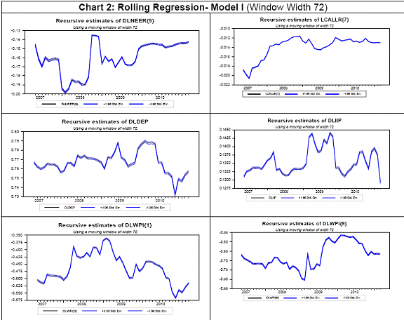
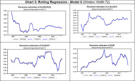
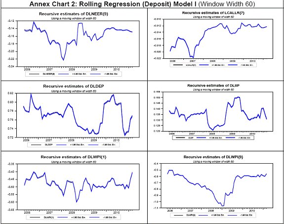
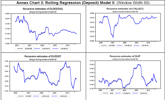
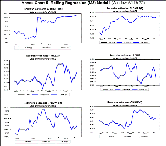
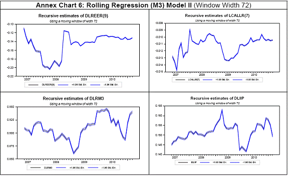
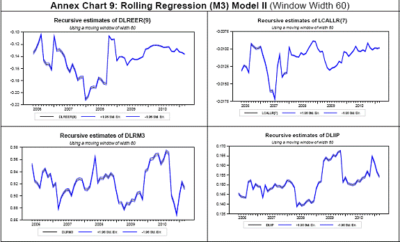
Further, Quandt-Andrews and Andrews-Ploberger tests for a single structural break at an unknown point within the sample also show that, in both the models, there is no structural break point for all the variables considered together. For the individual variables, however, both the tests in both the models show that only CallR has a statistically significant break in the coefficient at March 2009, i.e., about six months after the collapse of Lehman Brothers in September 2008 (Table-3). In other words, it appears that the global financial crisis led to a structural shift in the transmission of policy interest rate to the credit channel. 

More than the stability of the coefficients, our concern is on the lag structure and form of the equations, as our aim, from the monetary policy perspective, is to ascertain the consistency in the lag of policy transmission. However, it is highly plausible that the lag lengths of the explanatory variables, and the values and signs of the coefficients have undergone a transformation over various sub-sample periods due to change in underlying economic conditions. Consequently, sub-sample periods estimates could be significantly different from full sample period estimate in terms of lag structure of the explanatory variables. Thus, in order to confirm these, rolling regression technique was employed, primarily to check whether the coefficient of each of the variable, despite any changes in values, continued to maintain the same sign and remained statistically significant in all the sub-periods. The rolling regression coefficients with window width of 72 months for each of the variables along with +/- 1.96 standard error band representing statistical significance of these coefficients at 5 per cent level are presented in Chart 2 and 3 for the two models, respectively.

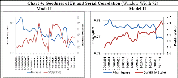
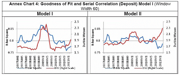
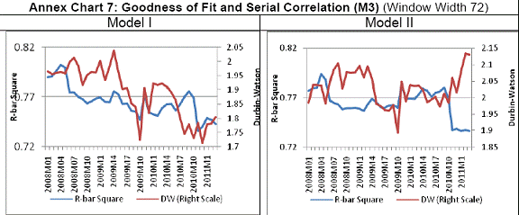
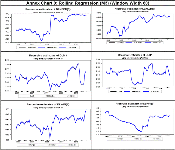
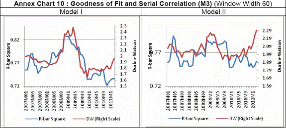
It can be seen that the value of all coefficients have undergone some changes over the sample periods, as reflected in the non-straight line charts. It is also observed that window size of the rolling regression does not significantly alter the shape of the charts⁵. However, what is important to our analysis is robustness of the estimates in terms of the sign and statistical significance of coefficients of all the variables.  Irrespective of window sizes and alternative form of models, the lag structure and signs of coefficients remain the same, and are also statistically significant in each of the sample period represented by each window. This statistical significance is shown by very close tracking of the coefficients by the two 5 per cent standard error bands indicating relatively low standard errors or high t-values. The goodness of fit measured by R-bar square ranges between 0.78 to 0.83 for Model I and between 0.76 to 0.82 for Model II, indicating high explanatory power. The serial correlations are also at acceptable levels with D-W statistics ranging from 1.62 to 1.86 for Model I and from 1.69 to 2.13 for Model II (Chart-4).

These results indicate that each of the variables has impacted bank credit in India with a consistent lag and in the same direction over the entire sample period, though the magnitude of the impact fluctuated over the sub-sample periods, barring the structural shift in the impact of policy rate. Particularly important from the monetary policy perspective is the result that the transmission lag of policy rate to both nominal and real credit channel has been consistently seven months, even though the magnitude of the impact got reduced somewhat in the post-Global crisis period.

V. Conclusions

The paper examined the operation of credit channel of monetary policy transmission in India through change in policy rate. The period considered was the post-LAF period of 2001:3 to 2011:3, when interest rate became the main instrument of signaling policy stance in India. The analysis was carried out through two reduced form equations drawn from the literature pertaining to nominal and real bank credit, respectively, and estimating regression equations based on them. The regression equations were estimated after transforming the variables into stationary form and following an approach similar to Hendry’s general-to-specific method. Specifically, controlling for other determinants, we estimated the lag impact of policy rate on the growth of both nominal and real bank credit. Besides the structural break tests, the consistency and robustness of the estimated equation in terms of lag structure of the variables across sub-sample periods were then confirmed by employing rolling regression technique.

The paper finds that nominal or real bank credit in India is contemporaneously influenced by the corresponding growth in economic activity and nominal or real deposit/money supply growth. It is thus implied that, besides the positive influence of economic activity on bank credit, policy induced expansion or contraction in deposit or money supply makes banks to adjust their credit portfolio correspondingly. Inflation and exchange rate appreciation have negative impact on the growth of bank credit with a long lag of nine months.

Importantly, from the point of view monetary policy perspective, the transmission of policy rate to nominal or real bank credit takes about seven months. This lag in transmission is found to be consistently true across various sub-sample periods obtained through rolling regression technique. During the full sample period under consideration, 100 basis points increase in policy rate was found to reduce the annualised growth in nominal and real bank credit by 2.78 per cent and 2.17 per cent, respectively.  However, it is found that there has been a statistically significant decline in the magnitude of the impact of policy rate on bank credit during the post global financial crisis period.

^@ Jeevan Kumar Khundrakpam is Director in the Monetary Policy Department.

^*These are strictly the personal views of the author.

¹It may be argued that segregation of the nominal income into its real and price component may give rise to problem of endogeneity among the explanatory variables. But, this segregation, as mentioned, is not only a common practice in the literature, but also enables identifying the difference in the size of elasticity between income and price.

²By considering the variables in real term and removing price variable from the explanatory variables, it also removes the problem arising from possible endogeneity between income and price variable.

³Estimated correlation coefficients between the explanatory variables revealed weak correlations between them ranging from 0.00 to 0.20 and were not statistically significant in almost all at the 5.0 per cent critical level.

⁴All the following reported results in the main text pertain to deposit growth, while all the other remaining results are presented in the Annex.

⁵ The corresponding rolling regression with window width of 60 is given at Annex.

References

Bernanke, B.S. and Blinder, A.S. (1988), “Credit, Money and Aggregate Demand”, American Economic Review, May, pp. 435-39.

Bernanke, B.S. and Blinder, A.S. (1992), “The Federal Funds Rate and the Channels of Monetary Transmission”, American Economic Review, September, pp. 901-921.

Bhaumik S.K., Vinh Dang and Ali M. Kutan (2010), “Implication of Bank Ownership for the Credit Channel of Monetary Policy Transmission: Evidence from India”, University of Michigan, William Davidson Institute Working Paper No. 988, May.

Cuikerman, A. and Hercowitz, Z. (1989), “Oligopolistic Financial Intermediation, Inflation and the Interest Rate Spread”, Foerder Institute for Economic Research, Tel Aviv University, Working Paper No.17-89.

Diamond, D. (1984), “Financial Intermediation and Delegated Monitoring”, Review of Economic Studies 51, 393-414.

Ehrmann, M., Leonardo G., Jorge Martinez-Pages, Patrick S. and Andreas W. (2001), “Financial Systems and the Role of Monetary Policy Transmission in the Euro Area”, European Central Bank Working Paper Series No. 105, December.

Gertler, M. and Gilchrist, S. (1993), “The Role of Credit Market Imperfections in the Monetary Transmission Mechanism: Arguments and Evidence”, Scandinavian Journal of Economics, Vol. 95, No.1, pp. 43-64.

Gertler, M. and Gilchrist, S. (1994), “Monetary Policy, Business Cycles, and the Behaviour of Small Manufacturing Firms”, Quarterly Journal of Economics, May, pp. 309-40.

Kashyap, A.K. and Stein, J.C. (1995), “The Impact of Monetary Policy on Bank Blance Sheets”, Carnegie-Rochester Conference Series on Public Policy, 42, pp.151-195.

Marsh, P. (1982), “The Choice Between Equity and Debt: An Empirical Study”, The Journal of Finance, Vol. 37, No.1, pp. 121-144.

Oliner, S. and Rudebusch, G.D. (1994), “Is There a Broad Credit Channel for Monetary Policy?”, Board of Governors of the Federal Reserve System, Research Working Paper, January.

Pandit, B.L. Ajit Mittal, Mohua Roy and Saibal Ghose (2006), “Transmission of Monetary Policy and the Bank Lending Channel: Analysis and Evidence for India”, Reserve Bank of India, Development Research Group Study No. 25.

Pandit, B.L. and Pankaj Vashisht (2011), “Monetary Policy and Credit Demand in India and Some EMEs”, Indian Council for Research on International Economic Relations, Working Paper No.256, May.

Romer, C.D. and Romer, D.H. (1990), “New Evidence on the Monetary Transmission Mechanism”, Brookings Papers on Economic Activity, No. pp. 149-213.

Vera, Leonardo V. (2003), “The Demand for Bank Loans in Venezuela: A Multivariate Cointegration Analysis”, Investigation Economica, Vol. LXII, No. 245, July-September.

Virmani Vineet (undated), “Examination of Credit Channel of Monetary Transmission in India: Results from response of commercial banks’ balance sheet to a monetary policy shock”, Indian Institute of Management, Ahmadabad (Mimeo).

Annex