 IST,
IST,
RBI WPS (DEPR): 01/2017: How Asset Prices Interact with Bank Credit and Monetary Policy? Evidence from Emerging Market and Developing Economies
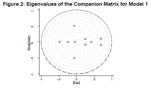
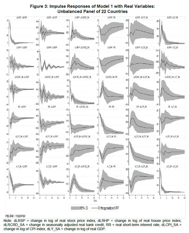
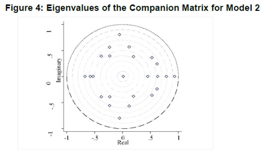
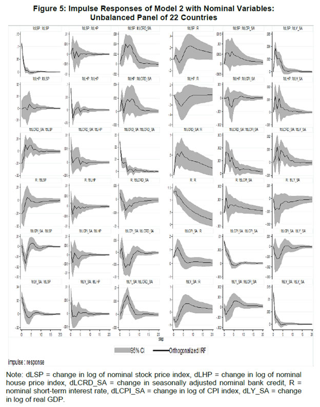
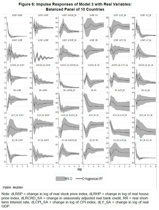
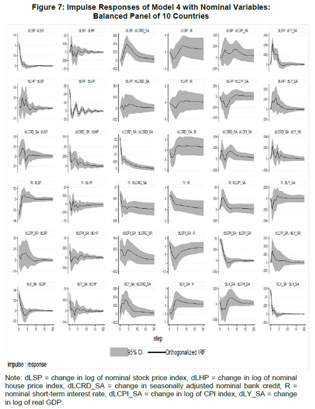
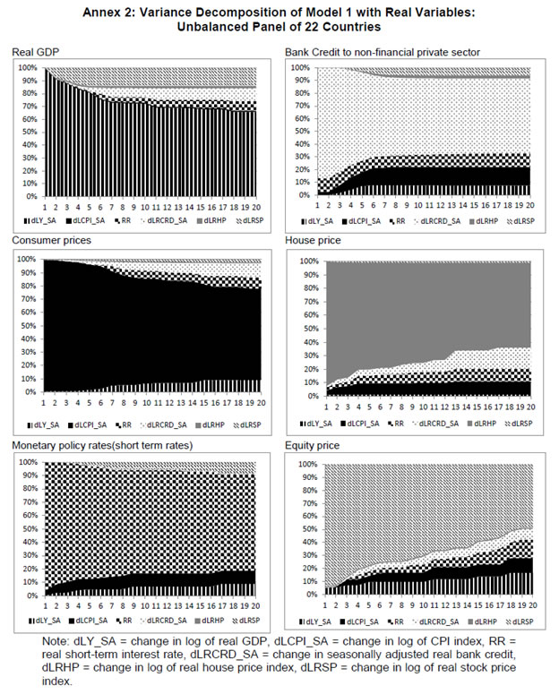
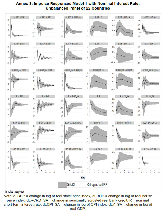
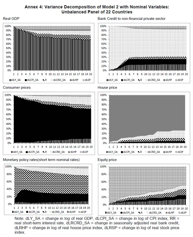
| RBI Working Paper Series No. 01 Abstract *The central hypothesis examined in this paper is whether credit shocks are more dominant in affecting asset prices vis-a-vis monetary policy shocks. The paper examines interaction of equity and house prices with macroeconomic factors using a panel VAR framework. Estimated models reveal dominance of monetary policy shock in causing fluctuations in stock prices, while bank credit shock plays greater role in driving house prices. Second, credit shock has sizeable and persistent impact on house prices in contrast to insignificant effect on stock prices. Third, a contractionary monetary policy shock causes decline in both real stock and house prices but the effect is relatively sizeable and persistent on equity prices as policy tightening could turn leverage costlier. JEL Classification: G12; E51; E52; E44 Key words: Asset Prices, Bank Credit, Monetary Policy, Financial Markets Introduction Asset prices have emerged as an important factor influencing allocation of credit and financial resources across sectors, impacting financial stability and driving fluctuations in business cycles i.e., output, employment and inflation. Notably equity and house prices, have exhibited significant fluctuations since the early 1980s, with a series of episodes of alternating boom-bust cycles both in advanced and emerging market economies. There is proliferation of empirical work in the context of advanced economies (AEs) establishing that asset price movements lead to significant changes in household wealth and thus impact their spending. The empirical evidence on wealth surprises causing medium to long-term shifts in spending behavior in AEs during the last two decades has mushroomed with asset prices cycles witnessing some of the longest expansionary as well as contractionary business cycles. Increasing globalisation and consequent integration of financial markets since the 1980s have been associated with significant shifts in the trajectory of asset prices and increasingly correlated movement of asset prices across countries with implications for financial sector and real economic activity. The experience of the asset price bubbles in Japan during the 1980s, Scandinavian countries (Finland, Norway and Sweden) during the 1980s and 1990s, East Asian countries in 1997-98 and the global financial crisis of 2008 suggest that significant trend divergence and persisting volatile movements in asset prices had disruptive effects on the financial and real sectors, engendering and prolonging global economic recessions. It is generally understood that rapid credit growth for extended periods coupled with large surges in asset prices may increase the likelihood of financial instability. The rising number of episodes and macroeconomic costs of financial instability in both the advanced economies and emerging markets since the 1980s have underscored the importance of asset prices in macroeconomic and policy discussions (see Bordo et al., 2001). Despite this, empirical work examining the relationship between credit and asset prices, or effect of changes in real estate prices on aggregate demand, is still quite limited (Borio and Lowe, 2002). Some notable empirical works on the relationship between credit and asset prices, inter alia, include Blundell-Wignall and Bullock (1993), Borio et al. (1994), Goodhart (1995), Hofmann (2001) and Goodhart and Hofmann (2008). The cross-country econometric tests of the relationship between asset price cycles and financial stability are limited and confined to equity prices (Borio and Lowe, 2002). However, Borio and Lowe (2003) argue that the source of financial instability cannot be solely ascribed to rapidly rising asset prices, rather it is a combination of increasing asset prices, rapid credit growth, and/or above average capital accumulation. They also find that when asset prices rise by 40-50 per cent from their trend and credit increases by 4-5 percentage points from its trend, 50 per cent of all financial distresses could be predicted with least amount of error. The variants of standard asset pricing models attempt to evaluate the present value of payoffs or cash flows discounted for risk and time lags. However, a key challenge posed by discounting process is the identification of relevant factors that affect payoffs. Against this backdrop, going beyond the standard asset price models of expected discount dividends, the aim of this study is to empirically explore the linkage between asset prices (viz., housing and stock prices) and macroeconomic aggregates in emerging market and developing economies (EMDEs), representing developing Asia, emerging Europe, Africa and Latin America. In this study, we seek to answer the question how bank credit growth affects asset price evolution and the relative dominance of the credit shocks over interest rate shocks in causing fluctuations in asset prices.1 Given the endogeneity and strong correlations between macroeconomic variables, there is a need for more work in the direction of understanding the common behaviour of short-term interest rates (signifying monetary policy), bank credit, asset prices and broad macroeconomic aggregates. This study attempts to contribute to the empirical aspects by using a panel VAR framework to examine the dynamic interaction between inflation, output, bank credit, monetary policy and house and equity prices for a cross section of 22 EMDEs, given that economies can no longer be treated in isolation due to greater global integration and common cycles impacting across EMDEs. As argued by Canova and Ciccarelli (2013), Panel VAR models have inherent advantages in terms of capturing both static and dynamic interdependencies, incorporating time variations in the coefficients and in the variance of the shocks, and in accounting for cross sectional dynamic heterogeneities. Section II sets out theoretical framework and debate on monetary policy, bank credit and asset prices and their feedback loops. Methodology used in the study is elaborated in Section III including identification schemes for various shocks. Section IV briefly discusses data issues and sources and empirical results obtained from the panel VAR model are discussed in Section V. Conclusion and policy issues are presented in Section VI. Central to the asset pricing theory is the notion that price of an asset equals expected discounted payoff. Following Cochrane (2001), the simplified form of an asset pricing model can be postulated as: pt = Et (mt+1* xt+1) (1) where the price of an asset (e.g., bonds, house or stock) at time t (pt) equals the expected value of the product of a stochastic discount fraction (mt+1) and payoff of the asset at time t+1 (xt+1). The above pricing equation holds for all asset classes. The real life asset price movements are, however, not that straightforward to comprehend due to numerous (unobservable) factors such as risk premia demanded by investors, specific distributional properties of price/return of a particular asset, international comovement of asset prices, the bubble-like behavior and liquidity constraints faced by a particular asset market. Capital Asset Pricing Model (Sharpe, 1964) provided an elementary framework to explain the relationship between asset prices and risk. It contends that a particular asset may require a higher return in compensation if it is correlated more strongly with the market as a whole. The model considers asset’s sensitivity to non-diversifiable risk (i.e., systematic risk or market risk), often represented by the quantity beta (β), and the expected return of the market and the expected return of a theoretical risk-free asset: ra = rf + βa (rm – rf) (2) where ra = expected return on an asset, rf = risk free return, βa = Beta of the security, rm = expected return of the market. Further theoretical frameworks examining the relationship between asset price movement and macroeconomic variables is provided by the dividend discount models (Gordon, 1959) and the arbitrage pricing theory (Ross, 1976). These theoretical frameworks suggest that new information or news of macroeconomic factors may impact the returns on stocks through their impact on expected dividend and discount factor. As the elementary dividend discount model implies that the value of an asset (PA) equals present value of expected future dividends, the latter should reflect real economic activity. Dividend Discount Model (Gordon,1959) is specified as: PAt = Dt+1 / [r-g] (3) Where PA is the current stock price, g is the constant growth rate in perpetuity expected for the dividends and r is the constant cost of equity capital for the firm and Dt+1 is the value of the next period dividends. Arbitrage Pricing Theory (Ross, 1976) holds that the expected return of a financial asset can be posited a linear function of various macroeconomic factors or theoretical market indices, where a factor-specific beta coefficient (bj) represents the sensitivity of asset return to changes in each factor (RP): E(rj) = rf + bj1RP1+ bj2 RP2 + bj3 RP3 + bj4 RP4 + ... + bj4 RPn (4) Where RP is the risk premium of the factor and rf is the risk-free rate. The model-derived rate of return is used for valuation of an asset. The asset price should equal the expected end of period price discounted at the rate implied by the model. If the price diverges, arbitrage should bring it back to the price valued by the model. The macroeconomic multifactor models associate stock return to factors such as interest rate, employment and inflation.2 Asset price fluctuations or prolonged deviations may emanate from factors such as information asymmetry and skewed allocation of credit or financial resources to some sectors or asset classes. When asset prices expand at a rate high than what can be justified by market fundamentals (Kindleberger, 1992). Ample debate has occurred that fundamentals alone may not be in a position to explain major variations in asset prices over shorter time horizons. A number of reasons have been identified, particularly in regard to deviation of stock prices from their (long-term) values, which primarily include expansion in credit, shifting of risks in financial system, herd behavior among market participants due to information asymmetry and overreaction or irrational response to economic news. Changes in credit growth is identified as an important factor causing significant variation in asset prices and amplification of business cycles. Relaxation in credit constraints can lead to changes in asset valuation either directly through purchases of real and financial assets or indirectly by increasing spending on goods and services, which may in turn enhance cash flows in the economy and brighten prospects of future income on assets holdings. Thus, a self-reinforcing cycle of credit and asset price increases may set in motion with higher credit growth fuelling asset prices, which in turn relaxes the credit constraint further. Some studies have also highlighted the speculative aspects of asset price formation with investment in assets increasingly guided by the expected valuation gains rather than return from investment in asset (Kindleberger, 1978; Minsky, 1982). When rising asset valuations are disconnected from the underlying macroeconomic fundamentals for a prolonged period, collapse in asset prices set in motion with painful adjustments in the balance sheets of overleveraged financial entities and borrowers and declining and negative credit growth (Borio, Kennedy and Prowse, 1994). In this backdrop, we further analyse the two key financial factors underlying the asset price dynamics. II.1. Monetary Policy and Asset Prices The standard interest rate channel of monetary transmission suggests that monetary policy by altering real short-term interest rate influence firm investment and household spending on durable goods whereas credit channel operates by altering access of firm and household to bank credit. The standard asset price channel suggests that asset prices respond to monetary policy changes and consequently impact output, employment and inflation. Tobin’s q theory in fact lays out the framework under which monetary policy affects economy through its effect on equity valuations. When market value of a firm is high, it can increase investment spending by issuing lesser equity. In a monetarist framework, a reduction in money supply leads to a reduction in the money available to public for spending, leading to a cutback in their spending on equities and thus, lowering their demand and prices. Another channel is that contractionary monetary policy by lowering equity prices leads to erosion in household wealth, which in turn reduces consumption and aggregate output. Thus, for central banks it is important to assess the potential consequences of large and enduring asset price movements. Mishkin (2007) argues that policy makers need to understand the role housing plays in the monetary transmission mechanism if they want to set policy instruments appropriately to achieve dual goals of price stability and employment. Several studies have emphasised the importance of understanding the link between monetary and credit developments and their usefulness as early indicators of building up of financial imbalances (see Borio and Lowe, 2002 and 2004; Issing, 2002; Detken and Smets, 2004; Machado and Sousa, 2006; Adalid and Detken, 2007; Gerdesmeier, Reimers and Roffia, 2009). Asset prices directly or credit and leverage as lead indicators of asset prices may assume importance for the monetary policy given that credit bubbles and excessive leverage have been recognized as the driving forces underlying the buildup of asset price cycles. II.2. Bank Credit and Asset Prices With asymmetric information and adverse selection problems, equity assumes an important role as collateral for lending to alleviate the information asymmetry and associated problems, which in turn, enhances the supply or availability of loans and therefore, improves prospects of investment and influences asset prices (see Kiyotaki and Moore, 1997; Kocherlakota, 2000; Boissay, 2001; Chen, 2001). The economic theory suggests that credit constrained firms or households use assets as collateral to finance their investments because their discounted future income stream cannot be collateralised. With appreciation of an asset, the value of collateral for borrowers increases, which in turn, leads to credit expansion and a rise in the demand for and prices of assets. Thus, given the significance of credit constraints and external finance in many industrial and emerging market economies, bank credit has been identified as an important factor driving asset prices, both equity and house prices. Kindleberger (1978) observed that historically boom and bust episodes in asset markets had been strongly connected with significant changes in monetary and particularly, credit aggregates. A number of empirical studies have established the role of credit in asset price determination (see Hofmann, 2001; Zhu, 2003; Davis and Zhu, 2004). Kaminsky and Reinhart (1999) based on their study of a wide range of crises for 20 industrial and emerging countries find financial sector liberalisation and significant credit expansion emerged as common harbinger to the crises. Lecat and Mesonnier (2005) while investigating house price developments in 18 industrial economies find real credit growth, along with short-term interest rate, as an important factor explaining house price. In Egert and Mihaljek (2007)’s study of the Central and East European economies, private credit growth emerged as more important factor than interest rate in driving real estate prices. It is also found that countries with absence of mortgage equity extraction and conservative lending practices, exhibit relatively weak link between bank credit and housing prices, while the impact of credit is observed to be much greater in countries with higher equity extraction and greater credit penetration (Tsatsaronis and Zhu, 2004). Borio and McGuire (2004), Detken and Smets (2004) and Bruggeman (2006) examine the role of credit growth and liquidity conditions in leading to asset price booms. Bruggeman (2006) based on a panel of 18 industrialised economies finds that one third of the periods of sustained excess liquidity have been followed by an asset price boom. In case of US, Adrian and Shin (2010) find a positive relationship between asset price changes, bank leverage and adjustments to the size of their balance sheets. Thus, phases of economic growth and sharp appreciation in asset prices are associated with a rise in bank leverage as banks purchase more assets, which, in turn, amplifies price increase and further strengthens bank balance sheets. II.3. Other Macro and Micro Factors The literature highlights key long-term determinants of house price as growth in household income (Abelson et al., 2005; Klyuev, 2008; Tsatsaronis and Zhu, 2004), shifts in demographics (Ahearne et al., 2005; Egert and Mihaljek, 2007; Fitzpatrick and McQuinn, 2004; Terrones and Otrok, 2004), tax incentives and real interest rates (Abelson et al., 2005; Egert and Mihaljek, 2007; Meen, 2002; Schnure, 2005) and availability of bank credit (Collyns and Senhadji, 2002; Fitzpatrick and McQuinn, 2004; Tsatsaronis and Zhu, 2004). The multifactor models of asset price movements have focused primarily on either microeconomic factors such as dividend earnings, PE ratios or the effect of global factors (viz., portfolio flows), thus, leaving macroeconomic determinants as less important or less explored.3 However, Bekaert and Harvey (1995) provide evidence that stock markets of emerging economies are less than perfectly integrated, which is a primary assumption of the international asset pricing model. Thus, a number of pricing factors may emerge significant in relatively less integrated emerging markets.4 The observed co-movements of share prices of firms tend to suggest presence of some exogenous variables which have a market-wide impact on prices. Particularly in the arbitrage pricing framework, macroeconomic factors are exploited to capture economy-wide risk factors (Burmeister and McElroy, 1988). In standard asset pricing models, macroeconomic factors that have significant impact on the expected cash flows or the discount factor, have important role in steering stock prices. Although, some suggest that the basis for selection of macroeconomic variables in explaining asset price movements is grounded on intuitive finance theory (McMillan, 2010), there are theoretical frameworks establishing a link between a particular macroeconomic variable and asset prices. The monetary portfolio theory suggest that volatility in money supply adjusts equilibrium position of money, thereby, changes the composition of an investor’s portfolio and the price.5 There are a few panel data based empirical studies for AEs and EMDEs establishing the relationship of stock prices with macroeconomic variables. Nasseh and Strauss (2000) find a long run association between economic activity and stock prices in European economies. It has been argued that inflation uncertainty, by impacting the discount rate, may affect the present value of future cash flows of firms. Boyd, Levine and Smith (2001) empirically observed a significant negative correlation between equity market activities and inflation rate. Fifield, Power and Sinclair (2000) in a study of 13 emerging stock markets discover that while world factors are significant in explaining the emerging stock markets returns, local factors (e.g., GDP, inflation, money and interest rates) are also equally important in explaining stock price movements. Nevertheless, there has not been any comprehensive attempt at examining the interaction among interest rate, bank credit and stock and house prices together for EMDEs. We attempt to bridge this gap in the empirical literature in the subsequent analysis. We explore the relationship between asset prices (i.e., stock and housing prices) and macroeconomic aggregates broadly following a conceptual framework similar to Goodhart and Hoffman (2008). A panel vector autoregression (PVAR) model is formulated to empirically examine the shocks that cause movements in house and equity prices and also to comprehend the role of asset price shocks in explaining fluctuations in key macroeconomic variables. The PVAR model conceptualised in this study blends the traditional VAR approach, which treats all variables in the system as endogenous, with the panel data approach that includes unobserved individual heterogeneity in the model. Panel VAR model in its structural form is specified as: A0Zit = Ai(L) Zit-1+ εit (5) where Z is the (m x 1) vector of endogenous variables of each of i countries, i = 1, …, N. Zit = (Z1t, Z2t,…, ZNt) for all countries. A0 is an (m x m) matrix with VAR coefficients and 1’s on the diagonal. It contains the structural parameters that capture the contemporaneous relationship among the endogenous variables. The disturbances, εit, are the vector with structural shocks with zero mean and a country-specific variance σN2. For the baseline model Zit = [yit, pit, rit, crit, Πit] and εit = [εyit, εpit, εrit, εcrit, εΠit], where y, p, r, cr and Π represent real output growth, consumer prices, real interest rate, real bank credit and real asset prices, respectively. Pre-multiplying equation (2) by A0−1, we obtain the following reduced form: Zit = B(L) Zit-k+ uit (6) where B(L) = A0−1A(L) and uit = A0−1εit which is a reduced form vector. The reduced form equation can be further modified to account for unobserved country effects and time effects. Our identification approach for recovering the structural parameters form the estimated reduced form equations involves imposing recursive zero restrictions on the contemporaneous structural parameters by applying Cholesky decomposition.6 The PVAR approach overcomes endogeneity issues and also allows for country-specific unobserved heterogeneity, largely absent in time series analyses. Estimation and inference is conducted in a generalized method of moments (GMM) framework.7 A consistent moment and model selection criteria for GMM models based on Hansen statistics of over-identifying restrictions has been proposed by Andrews and Lu (2001). However, it is considered that testing of over-identifying assumptions may not be essential in longitudinal applications given that time varying explanatory variables in different time periods are potential instruments. III.1. Identification of Shocks Theoretically plausible restrictions are imposed on the structure of the model to identify various structural shocks underlying fluctuations in asset prices. Typically, we need to impose the restriction so that matrices are the same for all cross sections (countries). Given that this assumption may be violated due to possible differences across EMDEs associated with a number of structural factors, our model can allow for individual heterogeneity in the levels of variables by introducing, say γi, to denote the fixed effects. The reduced form PVAR model enables us to estimate the unknown parameters. To identify the shocks, we use a Cholesky decomposition, with the variables ordered following the monetary policy VAR literature. In the identification scheme of shocks, we follow established practice in the literature of ordering real output and prices before interest rate as monetary policy reacts to both output and price changes (see Christiano and Gust, 1999). A triangular identification structure restricts all coefficients in the matrix to zero. A triangular identification structure imposed on the model indicated that output and price level respond only with a lag to monetary policy shocks, whereas there is contemporaneous/ instantaneous repose of bank credit, property and equity prices. It primarily captures aggregate demand shock with real GDP, consumer prices and nominal interest rate and asset prices increasing in response to the shock. It is argued that real GDP may also help capture that part of the demand for residential real estate that is driven mainly by the desire to consume housing services rather than investment considerations (Borio, Kennedy and Prowse, 1994). Given that equity prices are relatively volatile than housing prices, stock price shock could influence real income or output only with a lag (see Mishkin, 2008). Relatively volatile stock prices cause uncertainties in household decisions about consumption as they are not certain whether the shock will cause transitory or durable shifts in their wealth. Thus, stock wealth shocks may cause variations in real activity by increasing aggregate demand with some lag. Shock to consumer price is interpreted to mainly capture supply-side disturbances because as inflation rises, real GDP falls and nominal interest rate increases. We order short-term interest rate before bank credit and property and equity prices following bank credit. The short-term interest rate equation assumes in the form of the standard monetary policy reaction function wherein monetary policy reacts to output/real income and price shocks. Short-term interest rate variation are also reflective of expected changes in asset valuation. An important conduit from interest rate to asset prices is through the cost of mortgaged debt and thus demand for credit. Monetary policy changes can impact long-term cost of funds and have cascading effects on debt-financed housing demand and hence their market prices. To some extent, a similar pattern could also be observed underlying stock price fluctuations. Mishkin and White (2002), however, argue that most fluctuations in stock prices reflect real fundamentals or animal spirits, which are not related to monetary policy. Unlike Goodhart and Hofmann (2008), we include only credit and not money in the model. This, inter alia, helps avoid the model becoming very large and ensures identification of the structural disturbances since it is difficult to disentangle money and credit shocks due to close correlation between money and credit and credit being a subset of money (see Assenmacher-Wesche and Gerlach, 2008). Furthermore, unlike money, credit is recognised as an important variable that feeds a link for transmitting the effects of changes in asset prices on financial sector and real economy. Sharp and sustained credit growth combined with sizeable and prolonged increases in asset prices have played major role in many events of instability in the financial system (Hunter et al., 2003; Ahearne et al., 2005; Goodhart and Hofmann, 2007, 2008). Credit is ordered following short-term interest rate because credit demand may respond to changes in monetary policy rates. Furthermore, it looks appropriate to order credit before asset prices given the evidence of the role of bank credit in shaping asset price dynamics during the episodes of asset price booms and busts. The relationship between asset prices and credit may also turn out to be bidirectional - an increase in credit raising asset prices and higher asset prices facilitating relaxation of credit constraints. As the expectations of increasing income and the associated housing demand get entrenched, these lead to higher equilibrium prices of property and, hence, greater demand for bank credit. Thus, credit and asset price surges reinforce each other – reflecting a feedback loop.8 The reciprocal causation could emanate from the fact that credit growth induces investment in financial and non-financial assets. Rise in valuation of assets increases the valuation of collaterals which would, in turn, enhance the borrowing capacity of asset holders. 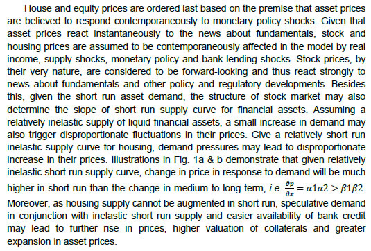 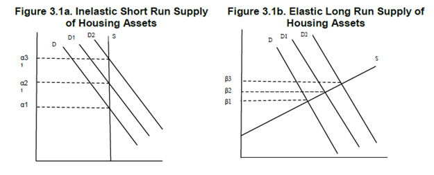 The period of the study is 1995:Q1 to 2014:Q4 to examine the dynamics of asset prices, credit and interest rates. A panel of 22 large EMDEs encompassing Africa, Asia, Europe and Latin America for which stock and house price data are available for a reasonable time period is considered for analysis, which inlcude Argentina, Brazil, Chile, China, Colombia, Croatia, Egypt, Hungary, India, Indonesia, Malaysia, Mexico, Nigeria, Pakistan, Peru, Philippines, Poland, Russia, South Africa, Thailand, Turkey and Venezuela. Since money and credit aggregates have high correlation and policy discussions are framed in the context of credit growth, we consider only bank credit in the model (see also Assenmacher-Wesche and Gerlach, 2008). Following variables are used in the model: real per capita income measured in terms of real per capita GDP at factor cost, consumer price index, real bank credit to private non-financial sector, i.e., nominal credit deflated by GDP deflator, real short-term interest, i.e., 3-month treasury bill yield or money market rate minus GDP deflator inflation, real house price i.e., nominal house price index deflated by GDP deflator, and real equity price, i.e., nominal equity price index deflated by GDP deflator.9 The secondary data sources used are World Bank online database, International Financial Statistics of IMF, BIS house price database, CEIC database, Haver Analytics, various central bank databases, national official statistics bureaus and other country-specific official data sources. The variable list, sample period and detailed data sources are presented in Annex 1. Summary statistics for variables used in the model is provided in Appendix Table 1. During the last one and a half decades, EMDEs have witnessed extended period of asset price growth and also deflationary cycles in asset prices (Table 1), making it interesting and challenging to understand their interaction with key macroeconomic factors. In this backdrop, the objective of this study is to investigate as to how credit growth and monetary policy changes interact with house and equity price movements. Bank credit, real GDP and CPI prices are seasonally adjusted. The panel stationarity test used for unbalanced panel for the period 1995:Q1 to 2014:Q4 reveals that all the variables included in our panel VAR have unit root, except interest rate, thus suggesting estimating models in first differences (see Appendix Table 2). We estimated the models with a lag order of four, which was selected based on the Akaike information criterion.10 We recover orthogonalised shocks based on a simple Cholesky decomposition with the following ordering: real GDP growth, inflation, interest rates, credit growth, house price changes and equity prices changes. These orthogonalised shocks should be interpreted as orthogonalised reduced form shocks rather than structural shocks as a particular shock will be unrelated to changes in other variables in the VAR system. Monte Carlo procedure is repeated 500 times and a 90 per cent confidence band is attained by computing 5th and 95th percentiles of the 500 bootstrapped impulse responses. V.1. Unbalanced Panel of 22 Countries: Model 1 with Real Variables We first estimate an unbalanced panel VAR model with six variables for the period 1995:Q1 to 2014:Q4 for a cross section of 22 EMDEs to examine the dynamic interlinkages among asset prices, credit and monetary policy.11 12 The fixed effect estimators are usually believed to be biased in panels that include lagged endogenous variables (see Holtz-Eakin, Newey and Rosen, 1988). With a view to overcoming this bias in estimation, we utilize GMM technique. The model is estimated using four lags decided based on various information criteria. The impulse responses derived from various models are generally different from zero at 95% confidence level as these are generated based on extensive information contained in panel data. We check for stability condition of the estimated panel VAR model. The eigenvalues in Figure 2 and Appendix Table 3 confirm that the estimates are stable as all the eigenvalues lie inside the unit circle. The impulse responses of real asset prices and key macroeconomic aggregates obtained from model 1 are presented in Figure 3 and Tables 2 and 3. Real GDP shock mainly captures the aggregate demand shock since real GDP growth, interest rate, credit demand and asset prices rise in response to the shock. An expansionary aggregate demand shock leads to significant increase in real credit growth, which persists for eight quarters.13 Simultaneously, there is significant increase in both house and equity prices. This, in fact, establishes the transmission from an expansionary aggregate demand shock to asset price appreciation through credit growth. The impact of aggregate demand shock on stock prices appears to be much more pronounced and durable as compared with the impact on house prices as evident from Table 3 and Figure 3. The impulse response functions reveal that a one percentage point increase in real GDP growth rate causes a peak increase in real credit growth of 0.54 percentage point, real appreciation of house price of 0.24 percentage point and a rise in real equity price of 1.95 percentage point (Tables 3). The impact on asset prices is instantaneous, which reemphasizes the sensitivity of asset prices to macroeconomic developments, with large contemporaneous impact on real equity prices as compared with house prices. Does monetary policy shock, i.e., an unanticipated increase in real policy rates, influence real asset prices? According to Mishkin (2007), interest rates can directly affect user cost of housing capital, expectations of future house-price movements as well as housing supply. It can also indirectly influence house prices through wealth effects, balance sheet and credit-channel effects on consumer spending and housing demand. The impulse responses in Figure 3 reveal that a contractionary monetary policy shock, by raising short-term interest rate, causes a (significant) instantaneous rise in real bank credit followed by a decline, which is accompanied by a decline in house and equity prices for one quarter. Given that asset prices are reflective of discounted value of future earnings, an increase in real interest rate should be associated with declining asset prices. The peak impact and accumulated impact of one unit shock to short-term interest rates in EMDEs, presented in Table 2 and 3, indicate that a contractionary monetary policy has much more sizeable (cumulative) impact on equity prices (-1.91 percentage point) than house prices (-0.36 percentage point). This may be due to two reasons. First, financial asset prices by their forward looking nature respond quickly through expectations channel and are, thus, more sensitive to changes in macroeconomic environment. Secondly, relatively lower magnitude of response of house prices as compared to equity prices in response to a monetary policy shock could also be due to lower size of mortgage market, underdevelopment leading to lower liquidity and limited ability of household to take equity out of housing assets. The overall findings score the point that monetary policy significantly influences asset prices in EMDEs and render support to the hypothesis that asset prices reflect a direct linkage with monetary policy changes rather than a common effect of a macroeconomic cycle. Thus, the inference that can be drawn from the foregoing analysis is that a contractionary monetary policy shock leads to a contraction in aggregate credit demand with a lag, which in turn, causes a contraction in the demand for financial and physical assets, thus setting in motion a cycle of lower demand and declining asset prices.14 Another key question that we strive to answer is whether real bank credit shock causes significant fluctuations in asset prices relative to monetary policy shock. Link between bank credit and asset price may work through wealth and collateral effects.15 Enhancement in availability of credit may augment demand for housing and financial assets provided households are credit constrained. Impulse responses generated by model 1 demonstrate that an expansionary bank credit shock leads to significant increase in the availability of bank credit and stimulates current and future economic activity (Figure 3). As bank credit boom signals an increase in real output, it raises expectations of future growth in corporate earnings and household incomes and, thus, leads to increases in both equity and house prices because of higher future returns. In our model an autonomous increase in real bank credit leads to an increase in real GDP which persists for three quarters. The impulse responses demonstrate that the impact of an expansionary real credit shock on house price persists for three quarters, whereas the impact on equity price, although positive, is found to be insignificant. While monetary policy shock has relatively higher impact on real equity price, bank credit shock has significant impact only on real house price. The phenomenon of lack of significant impact of credit shock on stock prices could be due to a number of factors such as sectoral credit controls i.e, regulatory restrictions imposed on bank credit for stock investments from the viewpoint of prudential regulation, significantly higher margin requirements on credit and less developed markets for collaterals based on equities. Our next question is that how macroeconomic variables respond to an asset price shock? Impulse responses in Figure 3 suggest that an expansionary exogenous shock to stock price leads to a significant increase in bank credit and is found to be persistent for six quarters. Enhancement of credit supply may occur through the effect of stock prices on the balance sheets of banks. By raising bank credit and investment demand, a positive stock price shock in turn leads to an expansion in real output which persists for about four quarters. A positive house price shock, through an increase in bank credit, leads to a rise in real output as well but the effect is not significant. Hofmann (2003), based on a panel analysis for AEs, find basically an accommodating role of bank credit in property-price cycles. Annex 2 presents variance decomposition of variables in the VAR model. For all the variables, fluctuations are largely explained by their own shocks. House price fluctuations are predominantly explained by its own shock. Monetary policy shock contributes about 9 per cent, inflation shock about 10 per cent and credit shock about 16 per cent of total fluctuations in real house prices over 20 quarters. Similarly, fluctuations in equity prices are predominantly explained by their own shocks. Aggregate demand shock explains about 17 per cent of total fluctuation in real stock returns, followed by 14 per cent by real interest rates over a period of 20 quarters, highlighting the important role of interest rate in evolution of financial asset prices. We also estimate a panel VAR model to analyse the impact of nominal monetary policy shocks (i.e, short-term nominal interest rate) on real asset prices in a panel VAR model of 22 countries with a view to find out if there are significant divergences in results when compared to the model with real policy shocks (Annex 3). To conclude, the impulse responses derived from the two models do not show any material differences. V.2. Unbalanced Panel of 22 Countries: Model 2 with Nominal Variables We also follow Goodhart and Hofmann (2008) framework to analyse the role of various shocks in explaining fluctuations in asset prices using nominal variables. We estimate the model with nominal variables (except for GDP) to understand differences in the interaction of nominal and real asset prices with macroeconomic variables. The ordering of variables and other assumptions of panel VAR Model 2 are the same as considered in Model 1. In what follows, we attempt to analyse the interaction between short-term nominal policy rates, nominal bank credit, and nominal house and stock price changes. The model is estimated with four lags chosen based on information criteria. First differences of all non-stationary variables are used except for interest rate. The estimates are stable as all eigenvalues lie inside the unit circle (Figure 4). Tables 4 and 5 present the peak impact, accumulated responses and persistence (lag effects) of variables to various shocks which fall within significant confidence bands. A comparison reveals that the persistence of nominal shocks seems to be somewhat longer than the persistence of real shocks (see Figure 5). The results from our GMM-based panel VAR reveal that an expansionary demand shock leads to an expansion in the nominal credit growth for about five quarters (cumulative 1.5 percentage point), which also leads to simultaneous increase in house and equity prices (Figure 5). As real output increases, there is short run moderation in inflation. It is important to note that cumulative impact of real output shock has sizeable impact on nominal equity prices (1.92 percentage point) than on nominal house prices (0.11 percentage point) since equity prices are considered to be more procyclical (Table 5). A contractionary monetary policy shock, measured in terms of an increase in short-term nominal interest rate, leads to moderation in real output growth. However, CPI inflation responds positively to a nominal interest rate shock, which can be attributed to the standard price puzzle. An initial jump in the nominal credit demand in response to contractionary monetary policy shock is followed by a significant decline persisting for about three quarters. Response of output remains the same as in the model with real variables. Nominal asset prices (both house and equity) respond negatively to a contractionary monetary policy shock but the impact is much more sizeable for equity prices (-6.1 percentage points cumulatively) as compared to house prices (-0.61 percentage point). Nominal monetary policy shock is found to cause strong contemporaneous changes in nominal equity prices, which reflects the procyclical behavior of financial asset prices. Thus, a contractionary nominal monetary policy shock causes simultaneous contraction in nominal bank credit, house and stock prices with greater persistence of shocks for credit demand. How do nominal credit shocks interact with macroeconomic aggregates and nominal asset prices? An expansionary nominal credit shock causes significant increase in real output which persists for a quarter and also results in a rise in nominal house price for about four quarters; impact on equity price is relatively insignificant as was observed in the model with real variables (see Figure 5). The asset price dynamics turns complicated as an expansionary credit shock leads to simultaneous increase in both output and asset prices. From a policy perspective, it becomes challenging to disentangle the fundamentals-led increase in asset prices from those induced by speculative credit flows. How does a nominal asset price shock affects macroeconomic aggregates? An exogenous expansionary shock to nominal equity price leads to significant expansion in credit demand for about 8 quarters and consequent expansion in real output (see Figure 5). Goodhart and Hofmann (2004) have contextually argued that financial sector liberalization may have fostered procyclical lending practices of banks which could have led to more procyclicality of financial systems. Positive nominal house price shocks are found to be persistent and cause significant but marginal increase in output without a significant impact on credit demand. Variance decomposition of the fluctuations of nominal asset prices and other macroeconomic variables is presented in Annex 4. A comparison of the variance decomposition of model 1 and 2 with real and nominal variables, respectively, reveals that movements in short-term interest rates are explained in relatively larger proportion by changes in CPI and bank credit in model 2, which implies greater response of monetary policy to inflation and bank credit growth. Secondly, output shock explains relatively greater fluctuations in nominal credit demand in the model 2 with nominal variables. Otherwise, the variance decomposition of real and nominal variables presented in Annex 2 and 4 do not exhibit any significant divergence. V.3. Balanced Panel of 10 Countries: Model 3 with Real Variables As part of the exercise to check the robustness and stability of results of panel VAR models, we recalibrate the above models using a balanced panel of 10 EMDEs over a shorter sub-sample (2000:Q1 to 2014:Q4) and compare the results with those obtained for the full sample period. The impulse responses generated by VAR model are presented in Figure 6. Impulse response functions suggest that there are no significant changes in the relationship between asset prices and macroeconomic variables in terms of direction and magnitude of impact between a smaller balanced panel (Fig. 6) and a larger unbalanced panel (Fig. 3). V.4. Balanced Panel of 10 Countries: Model 4 with Nominal Variables We also examine the response of nominal house and stock prices to important macroeconomic shocks for a balanced panel of 10 countries in order to understand variations in the bahaviour of nominal and real asset prices (Fig. 7). Two basic differences can be gleaned by comparing Fig. 5 and 7 for balanced and unbalanced panels, respectively. While in the unbalanced panel (22 countries) short-term interest rates, signaling monetary policy stance, witness an increase in response to nominal credit shocks, the response of monetary policy is not observed to be significant in the balanced panel (10 countries). Second, the persistence of interest rate shocks in reduced in the balanced panel. A comparison of real and nominal shocks in the balanced and unbalanced panel models reveals that persistence of nominal shocks is greater than that of real shocks. Secondly, the shocks are more persistent in the (broader) unbalanced panel than the (narrower) balanced panel. Otherwise, the results from both the balanced and unbalanced panel point to the similar macroeconomic dynamics. The response of asset prices to nominal and real shocks do not exhibit a significance divergence in the balanced and unbalanced panels. VI. Conclusion and Policy Issues The key inferences from our estimated benchmark panel VAR model with real variables for a sample of 22 countries are as follows: The principal shocks that influence movements in asset prices are real output (aggregate demand), bank credit and monetary policy shocks. First, real output shock, capturing mainly the aggregate demand shock, leads to significant increase in real credit growth, which persists for eight quarters after the initial shock. Simultaneously, there is significant increase in both house and stock prices - the impact on stock prices appear to be much more pronounced and durable as compared with the impact on house prices. A one percentage point increase in real GDP growth rate causes a peak impact of 0.54 percentage point increase in real credit growth, house price appreciation of 0.24 percentage point and rise in real equity price of 1.95 percentage points. The impact on asset prices is instantaneous, which re-emphasises the sensitivity of asset prices to macroeconomic developments, with large contemporaneous impact on real equity prices as compared with house prices. Second, real bank credit shock leads to significant increase in real output and a short run decline in inflation. Both real stock and house prices rise in response to an expansionary credit shock but the impact is significant and persistence only in the case of house prices. The phenomena of lack of significant impact on stock prices could be inter-alia attributed to various regulatory restrictions imposed on sectoral credit flow to stock markets. Third, a contractionary monetary policy shock leads to reduction in real output, which in turn, causes a decline in both real equity and house prices. The impact of monetary policy shock is found to be much more sizeable on equity prices than on house prices as tightening of monetary policy may turn the funding of leverage in financial markets costlier. A one unit contractionary monetary policy shock leads to a cumulative 1.91 percentage points decline in real stock prices whereas only 0.36 percentage point reduction in real house prices. Against the backdrop of our central hypothesis that credit shocks rather than interest rate shocks play important role in causing movements in asset prices, empirical results suggest that while bank credit shocks are more dominant in influencing real house prices, it is the monetary policy shock which primarily causes variations in real stock prices. House and equity prices respond at varying speeds and significantly varying magnitude to monetary policy shocks, signifying that it may turn out to be challenging for policy makers to simultaneously stabilise both. Second, aggregate demand shocks are found to be more dominant in causing fluctuations in asset prices as compared with credit shocks, thus highlighting the role of economic cycles in accentuating asset price rise. Equity price movements do not seem to be predominantly emanating from credit booms, which suggests that a major part of variation in credit growth is associated with expected variation in real economic activity. However, expansionary credit shocks rather than interest rate shocks trigger significant rise in house prices, which suggests an important role for macroprudential measures in dealing with asset prices rather than the interest rate policy. Empirical studies suggest that feedback from property prices to credit growth and the risk of a buildup of mutually reinforcing cycles in the real estate market is more pronounced in countries characterised by predominance of variable rate mortgages and market-oriented property price valuation systems (Tsatsaronis and Zhu, 2004). Borio and Lowe (2002) observe that sharp increases in asset prices and high credit growth together provide leading signals of financial instability. The impact of expansionary credit shock is more sizeable and persistence in case of house prices, suggesting the importance of monitoring large credit expansions, which may lead to excessive rise in banking system leverage and large asset price volatility. As EMDEs reach higher level of financial deepening, linkages between interest rate, credit, stock and house prices may turn stronger and the assessment of their effects may assume greater importance. The findings emerging from the foregoing analysis could have important policy implications for an EMDE like India. The limited role of credit shocks in causing stock price movements could be true for India given the regulatory norms for banks’ exposure to capital markets. Nevertheless, finding highlighting important role of credit in affecting house price movements, argues for the role of countercyclical macro-prudential polices in dealing with excessive house price movements. @ Bhupal Singh is Director in Monetary Policy Department of Reserve Bank of India (RBI), Mumbai. Avadhoot R. Nadkarni is former professor of economics, Department of Economics, University of Mumbai, Mumbai. Emails of the authors are bhupalsingh1@gmail.com and arnadkarni@gmail.com. *This paper is one of the three essays of the PhD dissertation submitted to the University of Mumbai by Bhupal Singh under his PhD supervisor Prof. A. R. Nadkarni. Authors would like to express deep gratitude to Michael Abrigo and Inessa Love of the Department of Economics, University of Hawaii for quick response to emails and readily sharing their Stata programme of Panel Vector Autoregression model used in this paper. Authors have benefitted from comments received from Prof. Neeraj Hatekar, Director and Professor of Econometrics of the Department of Economic, University of Mumbai as a discussant of the paper in a Seminar held at the Department of Economic and Policy Research (DEPR) of RBI on December 14, 2016. Authors gratefully acknowledge comments received from the seminar participants of DEPR Study Circle, RBI. Authors have also benefitted from the discussions on methodological aspects with Joice John of Monetary Policy Department on initial drafts. Without some critical panel data series made available by Indranil Sengupta of the Merril Lynch and Rohini Malkani and Anurag Jha of the Citi Group, some of the empirical exercises would not have been possible. The views expressed in the paper are solely of the authors and do not represent views of the respective institutions. 1 The study focusses on asset price cycles rather than bubbles. 2 These models compare two or more factors to analyze relationships between variables and equilibrium asset prices. 3 If markets are globally integrated, asset returns ought to be determined by a single priced global factor. However critical assumptions of this framework are that the markets should be fully integrated and the global benchmark portfolio must be mean-variance efficient. 4 According to the multifactor model, variables influencing future investment opportunities or consumption- investment decisions are priced factors in equilibrium (Merton 1973). 5 Fama (1981) suggests important role of economic activity and inflation in the analysis of stock market activity. 6 The Cholesky decomposition of the covariance matrix of the error terms, which imposes a recursive orthogonal structure (causal ordering) on the identified shocks is the most common method to overcome the identification problem. 7 PVAR model are estimated using GMM method in a multivariate panel regression framework wherein each dependent variable regressed on lags of itself and lags of all other dependent variables. 8 Theoretically, bank-lending channel may be particularly relevant for developing countries characterised by underdeveloped financial markets where interest rates may not move to clear markets. 9 There are issues regarding uniformity of the house prices across countries. While house prices for some countries are only for new dwellings, for most countries these include aggregate prices. 10 We use the Panel Vector Autoregression Stata programme of M. Abrigo and I. Love (2015). 11 In anticipation of distortion in the results, we use a dummy for the 2008 global financial crisis but find that there is no perceptible variation in the impulse responses. 12 The impact of country-specific institutional structure could be captured by segregating the sample into market-based and bank-based financial systems. Levine (2001) applied the ratio of value of domestic equities traded on domestic exchanges/GDP relative to the bank credit to private sector/GDP. 13 Impulse responses which are significant are taken into account and impulse responses with wide confidence bands, as they turn statistically significant, are ignored for interpretation. 14 We do not delve into the analysis of effects of monetary policy shock on inflation and output, as the focus is on asset prices. In a nutshell, a contractionary monetary policy shock leads to a rise in CPI inflation and the impact persists for about three quarters, which is also known as the ‘price puzzle’ (Bernanke and Blinder, 1992; Sims, 1992). In view of higher expected inflation due to exogenous shocks such as commodity price, central bank raises interest rate that could be co-terminus with increase in prices as the shocks may have already been built into the economy. An increase in policy rate may also lead to a rise in financing cost for firms, which also tends to raise inflation rate. 15 The lifecycle model argues that a permanent shift in housing wealth causes higher spending and borrowing when homeowners try to smooth out consumption over the life cycle. Thus, rising house prices induce homeowners to spend and borrow more by enhancing their borrowing capacity against higher valuation of housing collaterals References Abelson, P., R. Joyeux, G. Milunovich, and D. Chung (2005), “Explaining House Prices in Australia: 1970–2003”, Economic Record, 81: 96–S103. Abrigo, M. and I. Love (2015). Estimation of Panel Vector Autoregression in Stata: A Package of Programs, May. Adalid, R. and C. Detken (2007), “Liquidity Shocks and Asset Price Boom/Bust Cycles”, Working Paper No. 732, ECB. Adrian, T. and A. Shin (2010), “Liquidity and Leverage”, Journal of Financial Intermediation, 19 (3): 418-437. Ahearne, A., J. Ammer, B. Doyle, L. Kole and R. Martin (2005), “House Prices and Monetary Policy: A Cross-Country Study”, International Finance Discussion Paper No. 841, Board of Governors of the Federal Reserve System, Washington, DC. Andrews, D.W.K. and B. Lu (2001), “Consistent Model and Moment Selection Procedures for GMM Estimation with Application to Dynamic Panel Data Models”, Journal of Econometrics, 101: 123-164. Arellano, M. and S. Bond (1991), “Some tests of specification for panel data: Monte Carlo evidence and an application to employment equations,” Review of Economic Studies, 58: 277-297. Arellano M. and O. Bover (1995), “Another look at the instrumental variable estimation of error component models,” Journal of Econometrics, 68: 29-51. Assenmacher-Wesche, Katrin and Stefan Gerlach (2008), “Monetary policy, asset prices and macroeconomic conditions: a panel-VAR study,” Working Paper 149, National Bank of Belgium. Bekaert, G. and C. Harvey (1995), “Time-varying world market integration”, Journal of Finance, 50: 403-444. Bean, C. (2003), “Asset Prices, Financial Imbalances and Monetary Policy: Are Inflation Targets Enough?” BIS Working Paper No.140, September. Bernanke B. S. and A. S. Blinder (1992), “The Federal funds Rate and the Channels of Monetary Transmission,” American Economic Review, 82: 901-921. Bernanke B. S. and M. Gertler (1999). “Monetary policy and asset volatility”, Federal Reserve Bank of Kansas City Economic Review, 84(4): 17-52. Bernanke B. S. and A. S. Blinder (2001), “Should Central Banks Respond to Movements in Asset Prices”, American Economic Review, 91(2): 253-257. Blinder, A. S. and R. Reis (2005), “Understanding the Greenspan standard”, paper presented at the symposium ‘The Greenspan era: lessons for the future’, sponsored by the Federal Reserve Bank of Kansas City, Jackson Hole, Wyoming, August. Blundell-Wignall, A. and M. Bullock (1993), “Changes in the characteristics of the Australian business cycle: some lessons for monetary policy from the 1980s and early 1990s”, in Changes in the business cycle and the implications for monetary policy, BIS, April. Boissay, F. (2001), “Credit Rationing, Output Gap, and Business Cycles”, ECB Working Paper 87. Bordo, M. D., B. Eichengreen, D. Klingebiel and M. S. Martinez-Peria (2001), “Financial crises: lessons from the last 120 years”, Economic Policy, 32: 51-82. Bordo, M. D. and O. Jeanne (2002), “Monetary Policy and Asset Prices: Does Begin Neglect Make Sense?” International Finance, 5(2): 139-164. Bordo, M. D., M. J. Dueker and D. C. Wheelock (2002), “Aggregate price shocks and financial stability: a historical analysis”, Economic Inquiry, 40(4): 521-38. Bordo, M. D., M. J. Dueker and D. C. Wheelock (2003), “Aggregate price shocks and financial stability: the United Kingdom, 1796-1999”, Explorations in Economic History, 40(2): 143-69. Borio, C., N. Kennedy and S. Prowse (1994), “Exploring aggregate asset price fluctuations across countries: measurement, determinants and monetary policy implications”, BIS Economic Papers No 40. Borio, C. and P. Lowe (2002), “Asset prices, financial and monetary stability: exploring the nexus”, BIS Working Papers No 114. Borio, C. and P. Lowe (2003), “Imbalances or “bubbles”? Implications for monetary and financial stability”, in Hunter, Kaufman and Pomerleano (eds), Asset price bubbles, 247-270. Borio, C. and P. Lowe (2004), “Securing sustainable price stability: should credit come back from the wilderness?” BIS Working Paper, No 157. Borio C. and P. McGuire (2004), “Twin peaks in equity and housing prices?” BIS Quarterly Review, 79-93, March. Boyd, J. H., Levine, R. and B.D. Smith (2001), “The impact of inflation on financial sector performance”, Journal of Monetary Economics,” 47(2): 221-248. Burmeister, E., and McElroy, M. (1988), “Joint estimation of factor sensitivities and risk premia for the arbitrage pricing theory”, Journal of Finance, 38: 721-735. Bruggeman, A. (2006), “Can excess liquidity signal an asset price boom?” BIS Autumn Economists’ Meeting, 30-31 October, Basel. Canova, F., Ciccarelli, M. (2013), “Panel Vector Autoregressive models: A survey”, European Central Bank Working Paper 1507. Cecchetti S. G., H. Genberg, J. Lipsky and S. Wadhwani (2000), “Asset prices and central bank policy”, Geneva Reports on the World Economy, Vol. 2, Geneva: International Center for Monetary and Banking Studies, London: Centre for Economic Policy Research, July. Chen, N., Roll, R. and Ross, S. (1986), “Economic forces and the Stock Market”, Journal of Business, 59: 383-403. Chen, N.K. (2001). “Bank Net Worth, Asset Prices and Economic Activity,” Journal of Monetary Economics, 48: 415-36. Christiano, L. J. and C. J. Gust (1999), “Taylor rules in a limited participation model”, Working Paper 9901, Federal Reserve Bank of Cleveland. Cochrane, J.H. (2001), Asset Pricing, Princeton University Press, 2001. Collyns, C. and S. Abdelhak (2002), “Lending Booms, Real Estate Bubbles, and the Asian Crisis”, IMF Working Paper 02/20, Washington, DC. Crockett, A. (1998), “Financial liberalisation and financial fragility”, IMF Working Paper WP/98/83, Washington, DC. Crockett, A. (2001), “Monetary policy and financial stability”, BIS Speeches, 13 February. Davis, P. and H. Zhu (2004), “Bank lending and commercial property cycles: some cross-country evidence”, BIS Working Papers, No 150. Detken, C. and F. Smets (2004), “Asset price booms and monetary policy”, ECB Working Papers, No 364, May. Egert, B. and D. Mihaljek (2007), “Determinants of house prices in Central and Eastern Europe”, BIS Working Papers, No 236. Fama, E. F. (1981), “Stock returns, real activity, inflation and money,” The American Economic Review, 71: 545-565. Fifield, S., D. Power and C. Sinclair (2000), “A study of whether macroeconomic factors influence emerging market share returns”, Global Economy Quarterly, 1: 315-335. Filardo, A. J. (2004), “Monetary Policy and Asset Price Bubbles: Calibrating the Monetary Policy Trade-offs”, BIS Working Papers, No. 155, June. Fitzpatrick, T. and K. McQuinn (2004), “House Prices and Mortgage Credit: Empirical Evidence for Ireland”, Research Technical Paper 5/RT/04, Central Bank and Financial Services Authority of Ireland. Gerdesmeier, D., H. E. Reimers and B. Roffia (2009), “Asset price misalignments and the role of money and credit”, ECB Working Paper No. 1068. Goodhart, C. (1995), “Price stability and financial fragility”, in K. Sawamoto, Z. Nakajima and H. Taguchi. (eds) Financial Stability in a Changing Environment, London: Macmillan, 439-510. Goodhart, C. and B. Hofmann (2004), “Deflation, credit and asset prices”, in: R. Burdekin and P. Siklos (eds), Deflation. Current and historical perspectives, Cambridge, UK: Cambridge University Press, 166-88. Goodhart, C. and B. Hofmann (2007), House Prices and the Macroeconomy: Implications for Banking and Price Stability, Oxford: Oxford University Press. Goodhart, C. and B. Hofmann (2008), “House Prices, Money, Credit and Macroeconomy”, ECB Working Paper No. 888, April. Gordon, Myron J. (1959), “Dividends, Earnings and Stock Prices”, Review of Economics and Statistics, 41(2): 99–105. Greenspan, Alan (2002), “Opening remarks in Rethinking stabilization policy”, a symposium sponsored by the Federal Reserve Bank of Kansas City, Jackson Hole, Wyoming, 29-31 August. Goodhart, C. (1995), “Price stability and financial fragility”, in K. Kawamoto, Z. Nakajima and H. Taguchi (eds) Financial Stability in a Changing Environment, Chapter 10, 439-510, Macmillan, London. Harvey, C.R. (1995), “Predictable risk and return in emerging markets,” Review of Financial studies, 8: 773-816. Hofmann, B. (2001), “The determinants of bank credit to the private sector in industrialised countries”, BIS Working Paper No 108, December. Hofmann, B. (2003), “Bank lending and property prices: some international evidence”, HKIMR Working Paper No. 22/2. Holtz-Eakin, D., W. Newey and H. S. Rosen (1988), “Estimating vector autoregressions with panel data”, Econometrica, 56(6): 1371-1395. Hunter, William C., Kaufman, George G. and Pormerleano, Michael (2003), Asset Price Bubbles: The Implications for Monetary, Regulatory, and International Policies. Cambridge, MA: MIT Press. International Monetary Fund (2006), “Asset Prices and the Business Cycle”, World Economic Outlook, IMF, Washington, DC. Issing, O. (2002), “Monetary policy in a changing economic environment,” Proceedings, Federal Reserve Bank of Kansas City, 183-205. Kaminsky, G. L. and Reinhart, C. M. (1999), “The Twin Crises: The Causes of Banking and Balance-of-Payments Problems”, American Economic Review, 89(3), pp. 473-500. Kennedy, N and P Andersen (1994), “Household saving and real house prices: an international perspective”, BIS Working Paper, No 20, January. Kindleberger, C.P. (1978). Manias, Panics and Crashes: A History of Financial Crises, New York: Basic Books. Kindleberger, Charles P (1992), “Bubbles” in P. Newman et al., (eds), London: Macmillan. Kiyotaki, N. and J. Moore (1997), “Credit Cycles”, Journal of Political Economy, 105: 211-248. Kocherlakota, N.R. (2000), “Creating Business Cycles through Credit Constraints”, Federal Reserve Bank of Minneapolis Quarterly Review, 24: 2-10. Klyuev, V. (2008), “What Goes Up Must Come Down? House Price Dynamics in the United States”, IMF Working Paper 08/187, Washington, DC. Lecat, R. and J. S. Mesonnier (2005), “What role do financial factors play in house price dynamics?” Banque de France Bulletin Digest, 134: 1-37, February. Levine, R. (2001), “International Financial Liberalization and Economic Growth”, Review of International Economics, 9(4): 688-702. Maclennan, D., J. Muellbauer and M. Stephens (1998), “Asymmetries in housing and financial market institutions and EMU”, Oxford Review of Economic Policy, 14(3): 54-80. Machado, J. F. and J. Sousa (2006), “Identifying asset price booms and busts with quantile regressions”, Working Papers W2006/08, Banco de Portugal. McMillan, D.G. (2010), “Present value model, bubbles and returns predictability: sector-level evidence”, Journal of Business Finance and Accounting, 37: 668-686. Meen, G. (2002), “The Time-Series Behaviour of House Prices: A Transatlantic Divide”, Journal of Housing Economics, 11: 1–23. Merton, R. (1973), “An intertemporal capital asset pricing model”, Econometrica, 41: 867-887. Mishkin, F. S. and E.N. White (2002), “U.S. Stock Market Crashes and Their Aftermath: Implications for Monetary Policy”, Asset Price Bubbles Conference, Federal Reserve Bank of Chicago and The World Bank, Chicago, April 23. Mishkin, F. S. (2007), “Housing and the Monetary Transmission Mechanism”, NBER Working Paper No. 13518. Mishkin, F. S. (2008), “How Should We Respond to Asset Price Bubbles?”, Wharton Financial Institutions Center and Oliver Wyman Institute's Annual Financial Risk Roundtable, Philadelphia, Pennsylvania, May 15. Minsky, H. P. (1982), Can ‘It’ Happen Again? Essays on Instability and Finance, Armonk, New York: Sharpe. Mukherjee, T. K. and Naka, A. (1995), “Dynamic relations between Macroeconomic Variables and the Japanese Stock Market: An application of a Vector Error Correction Model”, Journal of Financial Research, 2: 223-237. Nasseh, A. and J. Strauss (2000), “Stock prices and domestic and international macroeconomic activity: a cointegration approach”, Quarterly Review of Economics and Finance, 40(2): 229-245. Ross, S. (1976), “The arbitrage theory of capital asset pricing”, Journal of Economic Theory, 13 (3): 341–360. Roubini, N. (2006), “Why Central Banks Should Burst Bubbles”, International Finance, 9(1): 87–107. Schnure, C. (2005), “Boom-Bust Cycles in Housing: The Changing Role of Financial Structure”, IMF Working Paper No. 05/200, Washington, DC. Sharpe, William F. (1964), “Capital asset prices: A theory of market equilibrium under conditions of risk”, Journal of Finance, 19(3): 425–442. Sims, C. (1992), “Interpreting the Macroeconomic Time Series Facts: The Effects of Monetary Policy”, European Economic Review, 36: 975-1011. Terrones, M. and C. Otrok (2004), “The Global House Price Boom”, IMF World Economic Outlook, September 2004, Washington, DC. Tsatsaronis, K. and H. Zhu (2004), “What drives housing price dynamics: cross-country evidence”, BIS Quarterly Review, March. Zhu, H (2003), “The importance of property markets for monetary policy and financial stability”, presented at the IMF/BIS Conference on Real Estate Indicators and Financial Stability, 27-28 October, Washington DC.
|
पृष्ठ अंतिम बार अपडेट किया गया:


